Simulation 3: ITS2 retrieval

library(RsemanticLibrarian)
library(LSAfun)
library(ggplot2)
library(ggcorrplot)
library(ggpubr)

Define some functions

row_H <- function(x){
  if(sum(x-x[1])==0) return(1)
  return(-1*sum(x*log2(x), na.rm=TRUE))
}

matrix_H <- function(x){
  return(mean(apply(x,1,row_H)))
}

sim_I <- function(x){
  max_error <- dim(x)[1]*dim(x)[2]*4
  # all ones matrix
  same_error <- sum((x - matrix(1,ncol=dim(x)[2],nrow =dim(x)[2]))^2)
  # identity matrix
  diff_error <- sum((x - diag(dim(x)[1])^2))
  
  return(log(same_error/diff_error))
}


higher_order_sim <-  function(x,range=1:5, graph=FALSE){
  if(graph==TRUE){
    cor_plots <- list()
    sim_save <- list()
    cor_plots[[1]] <- ggcorrplot(x, show.legend = FALSE)
    sim_save[[1]] <- x
  }
  informativeness <- sim_I(x)
  for(i in range){
    if(i ==1){
      higher <- cosine(x)
      informativeness <- c(informativeness,sim_I(higher))
      if(graph==TRUE) {
        cor_plots[[1+i]] <- ggcorrplot(higher, show.legend = FALSE)
        higher[is.na(higher)]<-0
        sim_save[[1+i]] <- higher
      }
    }else{
      higher <- cosine(higher)
      informativeness <- c(informativeness,sim_I(higher))
      if(graph==TRUE) {
        higher[is.na(higher)]<-0
        sim_save[[1+i]] <- higher
        cor_plots[[1+i]] <- ggcorrplot(higher, show.legend = FALSE)
      }
    }
  }
  
  if(graph==TRUE) return(list(informativeness,plots=cor_plots, sims=sim_save))
  if(graph==FALSE) return(informativeness)
}

frequency_matrix <- matrix(
  sample(1:100,10*100,replace=TRUE),
  byrow=TRUE,
  ncol=100,
  nrow=10
)

overlap <- matrix(0,ncol=100,nrow=10)
overlap[1, 1:15] <- 1
overlap[2, 11:25] <- 1
overlap[3, 21:35] <- 1
overlap[4, 31:45] <- 1
overlap[5, 41:55] <- 1
overlap[6, 51:65] <- 1
overlap[7, 61:75] <- 1
overlap[8, 71:85] <- 1
overlap[9, 81:95] <- 1
overlap[10, c(1:5,91:100)] <- 1

frequency_matrix <- frequency_matrix*overlap
prob_matrix <- frequency_matrix/rowSums(frequency_matrix)
veridical_sims <- cosine(prob_matrix)

nth_similarity <- higher_order_sim(veridical_sims,1:5, graph=TRUE)

This piece is the function to generate sentences from the language to form the corpus.

# sentence generator function
generate_sentence <- function(num_to_make=100,
                              s_length_range= 4:10,
                              topics_to_sample = 1:10,
                              topic_prob = rep(.1,10),
                              prob_mat = prob_matrix){
  all_sentences <- list()
  for(i in 1:num_to_make){
    sample_topic <- sample(topics_to_sample,1, prob = topic_prob)
    sample_length <- sample(s_length_range)
    sample_sentence <- c(sample(1:dim(prob_mat)[2],sample_length,
                                replace=TRUE,
                                prob=prob_mat[sample_topic,]))
    all_sentences[[i]] <- sample_sentence
  }
  return(all_sentences)
}

Simulation

corpus <- generate_sentence(num_to_make=5000,
                             s_length_range= 10:20,
                             topics_to_sample = 1:10,
                             topic_prob = rep(.1,10),
                             prob_mat = prob_matrix)

environment <- diag(100)

## populate ITS memory

its_memory <- matrix(0,ncol=dim(environment)[2],nrow=length(corpus))
for(i in 1:length(corpus)){
  its_memory[i,] <- colSums(environment[corpus[[i]],])
}

all_results <- data.frame()
for(dw in c(.01,.1,.2,.3,.4,.5)){
  print(dw)
  training <- c(100,500,1000,5000)
  its_vector_list <- list()
  for(t in 1:length(training)){
    #print(t)
    semantic_vectors <- matrix(0,ncol=100, nrow=100)
    for(p in 1:100){
      probe <- environment[p,]
      activations <- cosine_x_to_m(probe,its_memory[1:training[t],])
      activations[activations !=0] <- 1
      echo1 <- colSums(as.numeric(activations)*(its_memory[1:training[t],]))
      activations <- cosine_x_to_m(echo1,its_memory[1:training[t],])
      activations[activations !=0] <- 1
      echo2 <- colSums(as.numeric(activations)*(its_memory[1:training[t],]))
      semantic_vectors[p,] <- normalize_vector(echo1)-(dw*normalize_vector(echo2))
    }
    the_cosines <- cosine(t(semantic_vectors))
    the_cosines[is.na(the_cosines)] <- 0
    its_vector_list$vectors[[t]] <- the_cosines
    its_vector_list$plot[[t]] <- ggcorrplot(the_cosines, show.legend = FALSE)
    its_vector_list$sims1[[t]] <- cor(c(the_cosines),c(nth_similarity$sims[[1]]))^2
    its_vector_list$sims2[[t]] <- cor(c(the_cosines),c(nth_similarity$sims[[2]]))^2
    its_vector_list$sims3[[t]] <- cor(c(the_cosines),c(nth_similarity$sims[[3]]))^2
    its_vector_list$sims4[[t]] <- cor(c(the_cosines),c(nth_similarity$sims[[4]]))^2
  }
  nth_df <- data.frame(sims = c(its_vector_list$sims1,
                              its_vector_list$sims2,
                              its_vector_list$sims3,
                              its_vector_list$sims4),
                     training = rep(training,4),
                     order = as.factor(rep(1:4, each=length(training))),
                     discrepancy =dw)
  all_results <- rbind(all_results,nth_df)
}

ITS_retrieval <- all_results
save(ITS_retrieval,file="ITS_retrieval.RData")

library(ggplot2)

load("ITS_retrieval.RData")

ITS_retrieval$discrepancy <- as.factor(ITS_retrieval$discrepancy)
ITS_retrieval$training <- as.factor(ITS_retrieval$training)

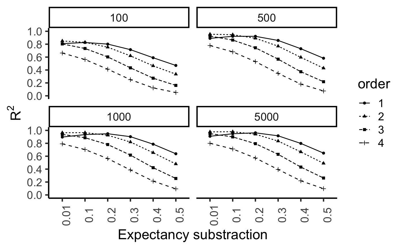
ggplot(ITS_retrieval, aes(x=discrepancy,y=sims, group=order, linetype=order,
                        shape=order))+
  geom_point()+
  geom_line()+
  xlab("Expectancy substraction")+
  ylab(expression(R^2))+
  scale_y_continuous(breaks=seq(0,1,.2))+
  coord_cartesian(ylim=c(0,1))+
  theme_classic(base_size=18)+
  theme(axis.text.x = element_text(angle = 90))+
  facet_wrap(~training)