Week 12: Tidy Tuesday example

This is an example of attempting a tidy tuesday challenge for May 2nd, 2023.

The data for this challenge is available at:

https://github.com/rfordatascience/tidytuesday/blob/master/data/2023/2023-05-02/readme.md

#install.packages("tidytuesdayR")

load libraries

library(tidyverse)

── Attaching packages ─────────────────────────────────────── tidyverse 1.3.2 ──
✔ ggplot2 3.4.1     ✔ purrr   1.0.1
✔ tibble  3.1.8     ✔ dplyr   1.1.0
✔ tidyr   1.3.0     ✔ stringr 1.5.0
✔ readr   2.1.4     ✔ forcats 1.0.0
── Conflicts ────────────────────────────────────────── tidyverse_conflicts() ──
✖ dplyr::filter() masks stats::filter()
✖ dplyr::lag()    masks stats::lag()

load data using the tidytuesdayR package

tuesdata <- tidytuesdayR::tt_load('2023-05-02')

--- Compiling #TidyTuesday Information for 2023-05-02 ----

--- There are 3 files available ---

--- Starting Download ---

    Downloading file 1 of 3: `plots.csv`
    Downloading file 2 of 3: `species.csv`
    Downloading file 3 of 3: `surveys.csv`

--- Download complete ---

plots <- tuesdata$plots
species <- tuesdata$species
surveys <- tuesdata$surveys

mice per year

mice_count_by_year <- surveys %>%
  group_by(year) %>%
  count()

ggplot(mice_count_by_year, aes(x= year, y=n))+
  geom_line() +
  geom_point()+
  ggtitle("Mice count by year")+
  scale_x_continuous(breaks=seq(1980,2020,5))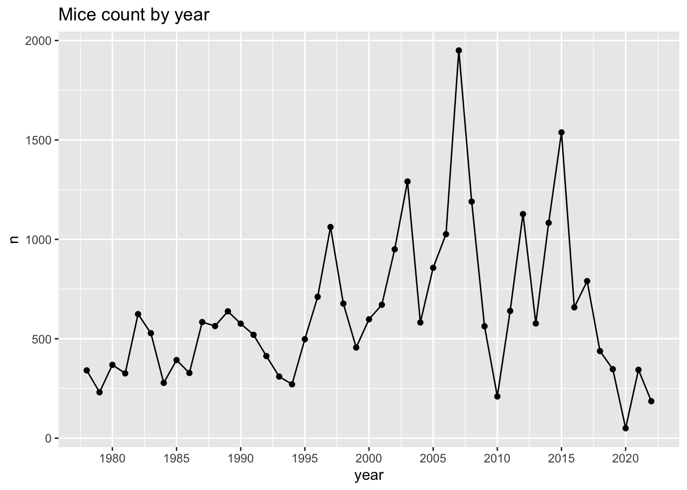

mice per year by sex

mice_count_by_year_sex <- surveys %>%
  group_by(year,sex) %>%
  count()

ggplot(mice_count_by_year_sex, aes(x= year, y=n, color=sex))+
  geom_line() +
  ggtitle("Mice count by year and sex")+
  scale_x_continuous(breaks=seq(1980,2020,5))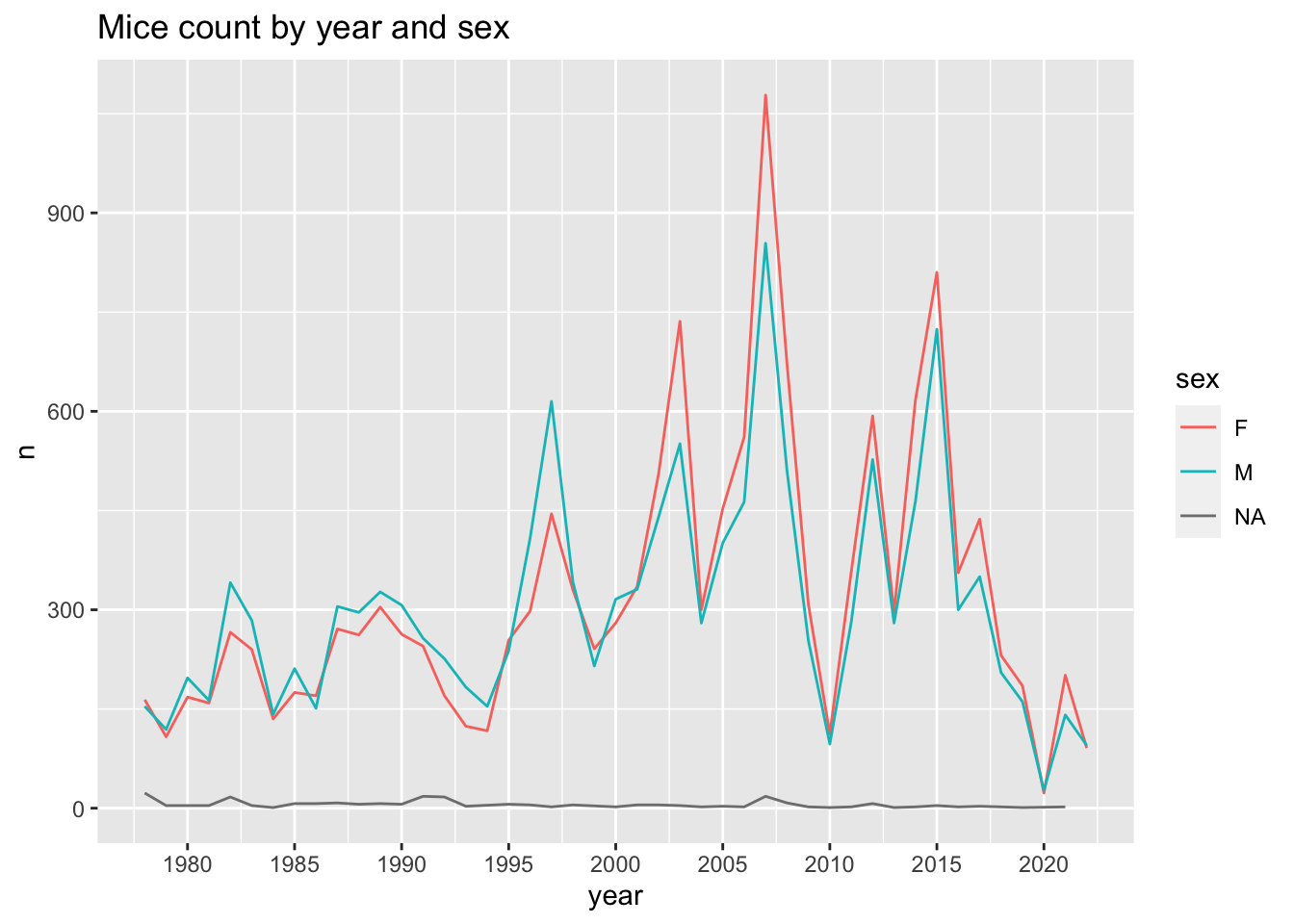

mice per year by species

mice_count_by_year_species <- surveys %>%
  group_by(year,species) %>%
  count()

ggplot(mice_count_by_year_species, aes(x= year, 
                                       y=n, 
                                       color=species,
                                       shape= species))+
  geom_line() +
  geom_point() +
  ggtitle("Mice count by year and species")+
  scale_x_continuous(breaks=seq(1980,2020,5))

Warning: The shape palette can deal with a maximum of 6 discrete values because
more than 6 becomes difficult to discriminate; you have 20. Consider
specifying shapes manually if you must have them.

Warning: Removed 321 rows containing missing values (`geom_point()`).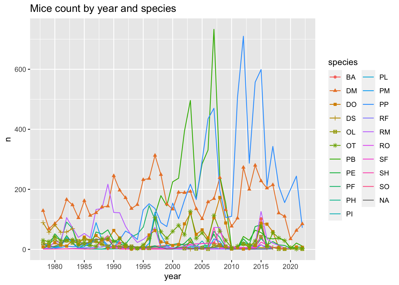

ggplot(mice_count_by_year_species, aes(x= year, 
                                       y=n, 
                                       color=species))+
  geom_line() +
  geom_point() +
  ggtitle("Mice count by year and species")+
  scale_x_continuous(breaks=seq(1980,2020,5)) +
  facet_wrap(~species)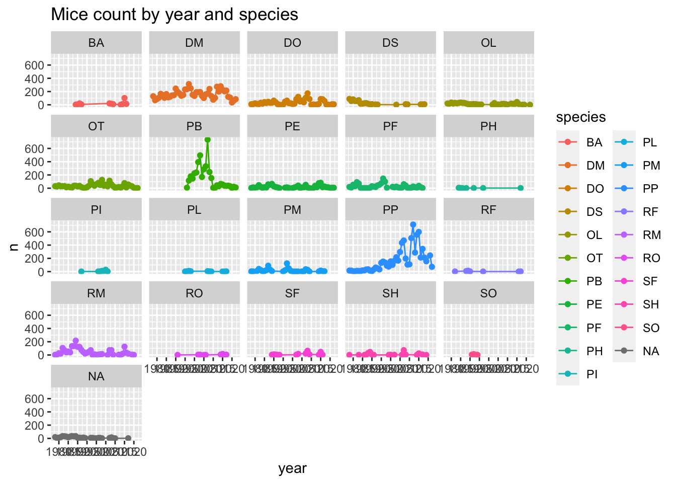

Pregnancy by month

monthly_data <- surveys %>%
  mutate(month_string = lubridate::month(censusdate,label= T)) %>%
  group_by(month) %>%
  count(pregnant) %>%
  pivot_wider(names_from=pregnant, values_from = n) %>%
  mutate(proportion_pregnant = P/(P+`NA`))

ggplot(monthly_data, aes(x=month, y=proportion_pregnant))+
  geom_line()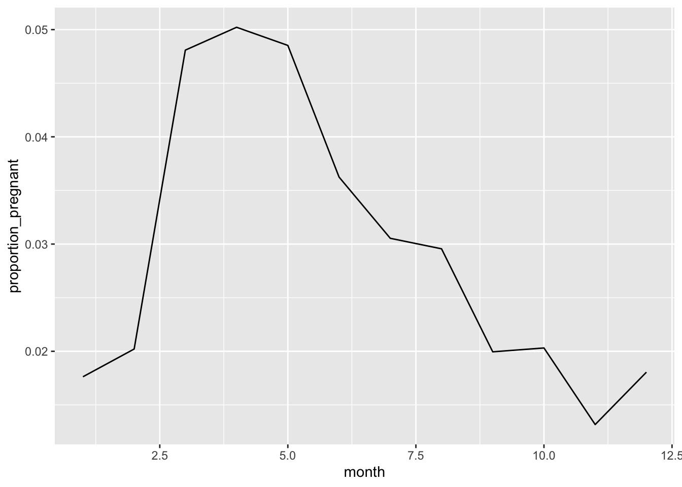

bob ross

tuesdata <- tidytuesdayR::tt_load('2023-02-21')

--- Compiling #TidyTuesday Information for 2023-02-21 ----

--- There is 1 file available ---

--- Starting Download ---

    Downloading file 1 of 1: `bob_ross.csv`

--- Download complete ---

#tuesdata <- tidytuesdayR::tt_load(2023, week = 8)

bob_ross <- tuesdata$bob_ross

ggplot(bob_ross, aes(x=num_colors))+
  geom_histogram()

`stat_bin()` using `bins = 30`. Pick better value with `binwidth`.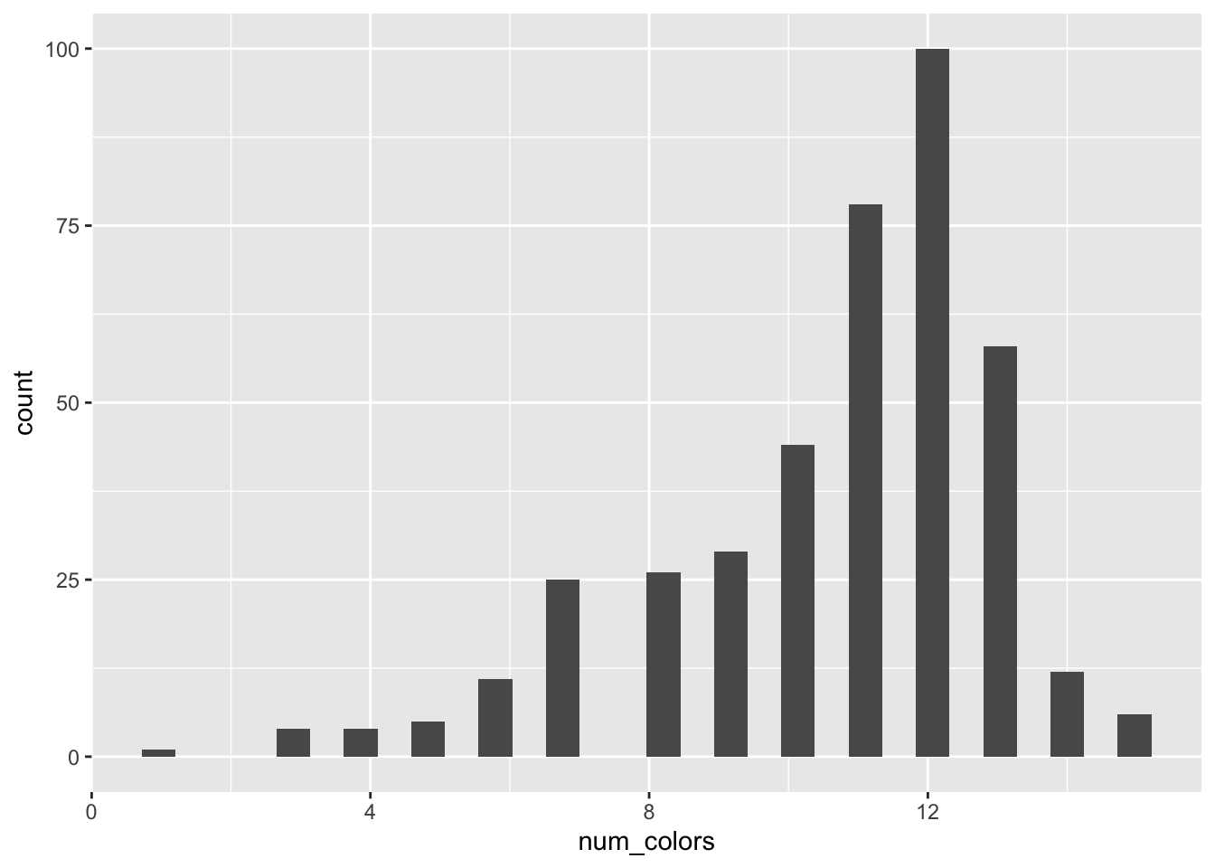

bob_ross_longer <- bob_ross %>%
  pivot_longer(10:27) %>%
  group_by(name) %>%
  summarize(count = sum(value))