week 7: more ggplot

library(tidyverse)

── Attaching packages ─────────────────────────────────────── tidyverse 1.3.2 ──
✔ ggplot2 3.4.1     ✔ purrr   1.0.1
✔ tibble  3.1.8     ✔ dplyr   1.1.0
✔ tidyr   1.3.0     ✔ stringr 1.5.0
✔ readr   2.1.4     ✔ forcats 1.0.0
── Conflicts ────────────────────────────────────────── tidyverse_conflicts() ──
✖ dplyr::filter() masks stats::filter()
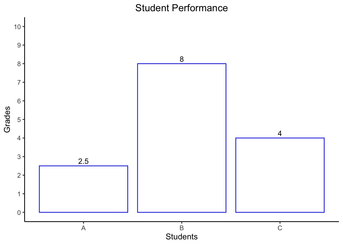
✖ dplyr::lag()    masks stats::lag()

grades <- c(2.5, 8, 4)
students <- c("A","B","C")
student_performance <- tibble(students,grades)

# alternate syntax

student_performance <- tibble(
  grades = c(2.5, 8, 4),
  students = c("A","B","C")
)

# ggplot bar graph
ggplot(student_performance, aes(x = students, y = grades))+
  geom_bar(stat = "identity", fill = "white", color = "blue") +
  scale_y_continuous(breaks = 0:10,limits = c(0,10)) +
  theme_classic() +
  geom_text(label=grades, position = position_dodge(width=.9), vjust=-0.4)+
  xlab("Students")+
  ylab("Grades") +
  ggtitle("Student Performance") +
  theme_classic(base_size = 12) +
  theme(plot.title = element_text(hjust = 0.5))

#Create a dataframe
factor_one <- rep(as.factor(c("A", "B", "C")), 2)
factor_two <- rep(as.factor(c("IIA", "IIB")), 3)
dv_means <- c(20, 30, 40, 20, 40, 40)
dv_SEs   <- c(4, 3.4, 4, 3, 2, 4)
plot_df <- data.frame(factor_one,
                      factor_two,
                      dv_means,
                      dv_SEs)

# basic bar graph

ggplot(plot_df,
       aes(
         x = factor_one,
         y = dv_means,
         group = factor_two,
         fill = factor_two
       )) +
  geom_bar(stat = "identity", position = "dodge")