Week 4 Datavis

A quick demo

1. Get some data in tidy data format
2. Understand what kind of data types you have in the dataframe so you can plot it appropriately
3. Graph the data with ggplot2

#loads ggplot2, and some example data sets
library(tidyverse)

── Attaching packages ─────────────────────────────────────── tidyverse 1.3.2 ──
✔ ggplot2 3.4.0     ✔ purrr   1.0.1
✔ tibble  3.1.8     ✔ dplyr   1.1.0
✔ tidyr   1.3.0     ✔ stringr 1.5.0
✔ readr   2.1.3     ✔ forcats 0.5.2
── Conflicts ────────────────────────────────────────── tidyverse_conflicts() ──
✖ dplyr::filter() masks stats::filter()
✖ dplyr::lag()    masks stats::lag()

# the starwars data is loaded by tidyverse
# assign the starwars dataset to a variable name
starwars_copy <- starwars

# check out some of the datatypes
head(starwars_copy)

# A tibble: 6 × 14
  name         height  mass hair_…¹ skin_…² eye_c…³ birth…⁴ sex   gender homew…⁵
  <chr>         <int> <dbl> <chr>   <chr>   <chr>     <dbl> <chr> <chr>  <chr>  
1 Luke Skywal…    172    77 blond   fair    blue       19   male  mascu… Tatooi…
2 C-3PO           167    75 <NA>    gold    yellow    112   none  mascu… Tatooi…
3 R2-D2            96    32 <NA>    white,… red        33   none  mascu… Naboo  
4 Darth Vader     202   136 none    white   yellow     41.9 male  mascu… Tatooi…
5 Leia Organa     150    49 brown   light   brown      19   fema… femin… Aldera…
6 Owen Lars       178   120 brown,… light   blue       52   male  mascu… Tatooi…
# … with 4 more variables: species <chr>, films <list>, vehicles <list>,
#   starships <list>, and abbreviated variable names ¹​hair_color, ²​skin_color,
#   ³​eye_color, ⁴​birth_year, ⁵​homeworld

class(starwars_copy$name)

[1] "character"

class(starwars_copy$height)

[1] "integer"

class(starwars_copy$mass)

[1] "numeric"

class(starwars_copy$homeworld)

[1] "character"

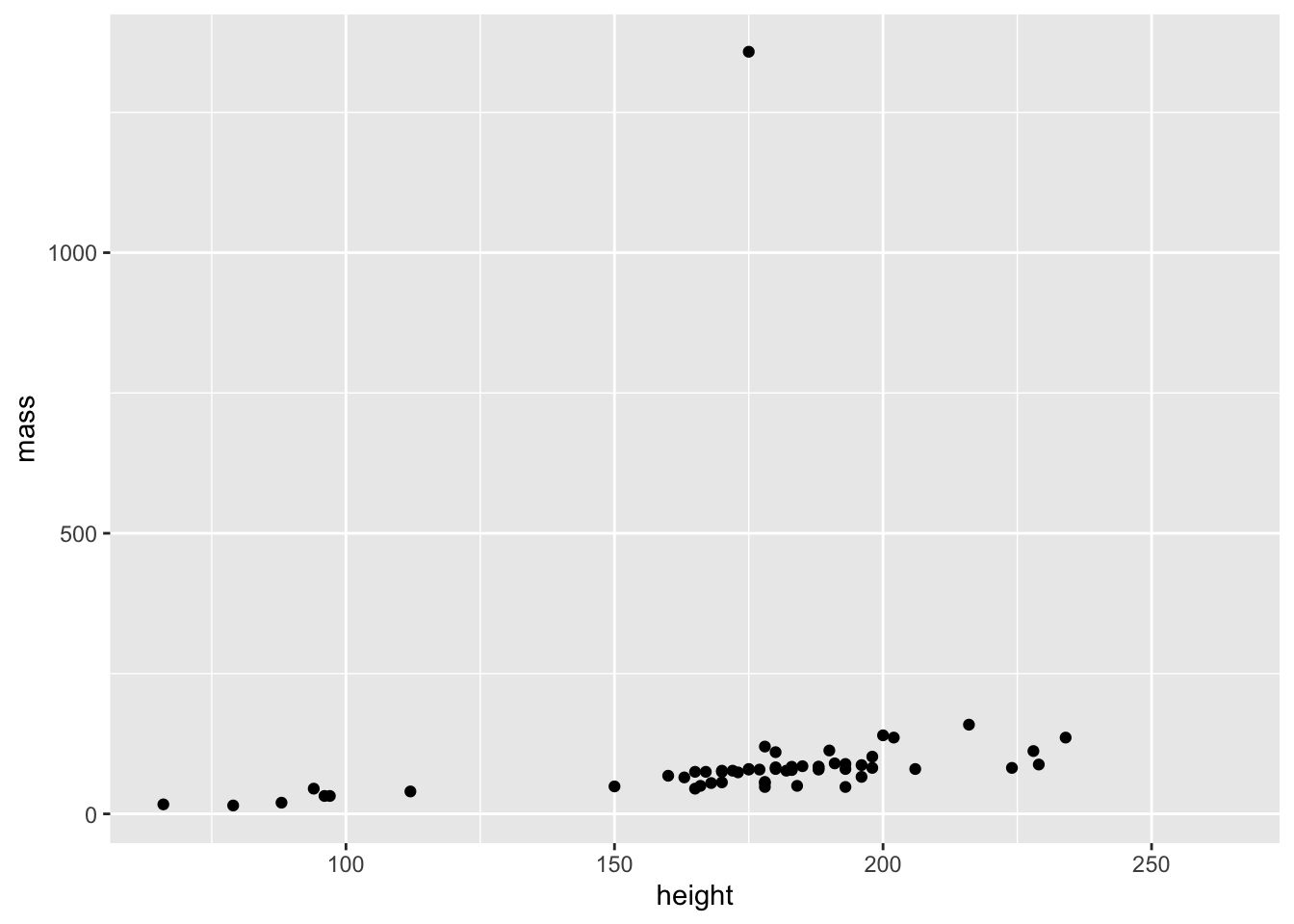
# plot some variables
ggplot(data = starwars_copy,
       mapping = aes(x=height,y=mass) )+
  geom_point()

Warning: Removed 28 rows containing missing values (`geom_point()`).

Data-types

What is in a name?

Everything is a function.

Object assignment

This is one of the simplest things you could do in R. What is happening here?

• a is the name of a new object that is being created

• <- is the assignment operator. It looks like an arrow, with the 1 going into the a

• 1 is an object that is being assigned into a

• consequences: a new object with the name a is created. This new object has been assigned the content 1.

# assign 1 to object named a
a <- 1
1 -> b

f <- 4 -> g

# look at the data type of object in a
class(a)

[1] "numeric"

typeof(a)

[1] "double"

Kinds of data types

Integers

#integers (no decimals)
# L specifies integer
typeof(1L) 

[1] "integer"

class(1L)

[1] "integer"

is.integer(1L)

[1] TRUE

as.integer(1.1) # coerces to integer

[1] 1

as.integer(1.5) # rounds down

[1] 1

as.integer(1.9) # rounds down

[1] 1

integer(length = 5) #initialize a vector for integers

[1] 0 0 0 0 0

is.integer(as.integer(1:5))

[1] TRUE

Numeric/doubles

# decimal numbers
# numbers without decimals default to numeric
typeof(1) 

[1] "double"

class(1)

[1] "numeric"

is.numeric(1)

[1] TRUE

as.numeric(1L) # coerces integer to numeric

[1] 1

numeric(length = 5) #initialize a vector for doubles

[1] 0 0 0 0 0

Character

Any text between quotes get’s treated as a character string

typeof("1") 

[1] "character"

class("1")

[1] "character"

is.character("1")

[1] TRUE

as.character(1) # coerces numeric to character

[1] "1"

character(length = 5) #initialize a vector for character strings

[1] "" "" "" "" ""

Logical/Boolean

Uppercase TRUE, or FALSE makes logical (binary) variables

typeof(TRUE)

[1] "logical"

class(TRUE)

[1] "logical"

is.logical(FALSE)

[1] TRUE

as.logical(1) # coerces 1 to TRUE

[1] TRUE

as.logical(0) # coerces 0  to FALSE

[1] FALSE

logical(length = 5) # initialize a logical vector

[1] FALSE FALSE FALSE FALSE FALSE

Object types

R has many object types to store individual elements, or collections of elements.

Vector

# makes a vector with one thing in it
one_thing <- 1
two_things <- c(1,2) 
many_things <- 1:100

data.frame

A table with rows and columns.

my_df <- data.frame(a = 1:5,
                    b = c("one","two","three","four","five"),
                    random = runif(5,0,1))
#print to see it
my_df

  a     b    random
1 1   one 0.4032073
2 2   two 0.1557925
3 3 three 0.2199378
4 4  four 0.3859071
5 5  five 0.5663455

# access columns with $
my_df$a == 1:5

[1] TRUE TRUE TRUE TRUE TRUE

my_df$b

[1] "one"   "two"   "three" "four"  "five" 

## access rows or columns with [row,column]
my_df[1,] # row 1, all columns

  a   b    random
1 1 one 0.4032073

my_df[,1] # column 1, all rows

[1] 1 2 3 4 5

my_df[1:2,] # rows 1 to 2, all columns

  a   b    random
1 1 one 0.4032073
2 2 two 0.1557925

my_df[1:2, 3] # rows 1 to 2, but only for column 3

[1] 0.4032073 0.1557925

Tibble

A table with rows and columns.

my_df <- tibble(a = 1:5,
                    b = c("one","two","three","four","five"),
                    random = runif(5,0,1))
#print to see it
my_df

# A tibble: 5 × 3
      a b     random
  <int> <chr>  <dbl>
1     1 one    0.882
2     2 two    0.156
3     3 three  0.752
4     4 four   0.863
5     5 five   0.767

# access columns with $
my_df$a

[1] 1 2 3 4 5

my_df$b

[1] "one"   "two"   "three" "four"  "five" 

## access rows or columns with [row,column]
my_df[1,] # row 1, all columns

# A tibble: 1 × 3
      a b     random
  <int> <chr>  <dbl>
1     1 one    0.882

my_df[,1] # column 1, all rows

# A tibble: 5 × 1
      a
  <int>
1     1
2     2
3     3
4     4
5     5

my_df[1:2,] # rows 1 to 2, all columns

# A tibble: 2 × 3
      a b     random
  <int> <chr>  <dbl>
1     1 one    0.882
2     2 two    0.156

my_df[1:2, 3] # rows 1 to 2, but only for column 3

# A tibble: 2 × 1
  random
   <dbl>
1  0.882
2  0.156

my_df

# A tibble: 5 × 3
      a b     random
  <int> <chr>  <dbl>
1     1 one    0.882
2     2 two    0.156
3     3 three  0.752
4     4 four   0.863
5     5 five   0.767

lists

Tidy data

Tidy data codes observations in a table. Each observation has its own row. The columns contain characteristics of the observation. For example, a demographics table could have one row per person, and several columns describing features of the person. Or, an expriment may involve multiple measures of a dependent variable across people and conditions of an independent variable. In this case, each row would contain one measurement, and each column would code the conditions associated with the measurement.

An example of wide vs. long data. In this example, the long-data is in tidy format. The accuracy measure is the dependent variable, and there is one row per measurement.

https://crumplab.com/programmingforpsych/dealing-with-data.html#standard-data-formats

ggplot2

library(tidyverse)
library(ggplot2)

survey_data <- read_csv("https://psyteachr.github.io/ads-v2/data/survey_data.csv")

Rows: 707 Columns: 7
── Column specification ────────────────────────────────────────────────────────
Delimiter: ","
chr  (3): caller_id, employee_id, issue_category
dbl  (3): wait_time, call_time, satisfaction
dttm (1): call_start

ℹ Use `spec()` to retrieve the full column specification for this data.
ℹ Specify the column types or set `show_col_types = FALSE` to quiet this message.

head(survey_data)

# A tibble: 6 × 7
  caller_id employee_id call_start          wait_time call_time issue_…¹ satis…²
  <chr>     <chr>       <dttm>                  <dbl>     <dbl> <chr>      <dbl>
1 C001      E01         2020-09-22 10:47:54       169        34 tech           3
2 C002      E01         2020-09-07 22:10:25       206        52 tech           2
3 C003      E01         2020-07-06 12:08:59       207        41 tech           2
4 C004      E01         2020-02-20 13:12:03       132        16 tech           4
5 C005      E01         2020-11-08 17:42:10       178        20 returns        3
6 C006      E01         2020-06-01 19:06:12       230        46 returns        2
# … with abbreviated variable names ¹​issue_category, ²​satisfaction

ggplot()

ggplot(data = survey_data,
       mapping = aes(x = wait_time,
                     y = satisfaction)
       )

ggplot(survey_data, aes(x = wait_time, y = satisfaction))

ggplot(survey_data, 
       aes(x = wait_time, 
           y = satisfaction)) + 
  geom_point()

ggplot(survey_data, 
       aes(x = wait_time, 
           y = satisfaction)) + 
  geom_point(color="red")

ggplot(survey_data, 
       aes(x = wait_time, 
           y = satisfaction)) + 
  geom_point(color="black", size = 5) +
   geom_point(color="#fa2fcb", size = 4) +
  geom_smooth(method ="lm")

`geom_smooth()` using formula = 'y ~ x'

ggplot(survey_data, 
       aes(x = wait_time, 
           y = satisfaction,
           color = wait_time,
           size = satisfaction)) + 
  geom_point()

min(survey_data$wait_time)

[1] 23

max(survey_data$wait_time)

[1] 314

length(survey_data$wait_time)

[1] 707

ggplot(data=survey_data, mapping= aes(x=wait_time))+
  geom_histogram(bins=50, color="red") +
  theme_classic()

change figure output size

ggplot(data=survey_data, mapping= aes(x=wait_time))+
  geom_histogram(bins=50, color="red") +
  theme_classic()

Random stuff I did in class

typeof(10.0245435234534)

[1] "double"

typeof(10L)

[1] "integer"

typeof(10)

[1] "double"

typeof("1")

[1] "character"

"one" < "two"

[1] TRUE

"z" < "w"

[1] FALSE

is.numeric(10)

[1] TRUE

is.numeric("1")

[1] FALSE

a <- c(1,2,3)
is.numeric(a)

[1] TRUE

is.numeric(starwars$name)

[1] FALSE

is.numeric(starwars$mass)

[1] TRUE

is.numeric(starwars$height)

[1] TRUE

is.integer(starwars$height)

[1] TRUE

class(starwars$height)

[1] "integer"

head(starwars)

# A tibble: 6 × 14
  name         height  mass hair_…¹ skin_…² eye_c…³ birth…⁴ sex   gender homew…⁵
  <chr>         <int> <dbl> <chr>   <chr>   <chr>     <dbl> <chr> <chr>  <chr>  
1 Luke Skywal…    172    77 blond   fair    blue       19   male  mascu… Tatooi…
2 C-3PO           167    75 <NA>    gold    yellow    112   none  mascu… Tatooi…
3 R2-D2            96    32 <NA>    white,… red        33   none  mascu… Naboo  
4 Darth Vader     202   136 none    white   yellow     41.9 male  mascu… Tatooi…
5 Leia Organa     150    49 brown   light   brown      19   fema… femin… Aldera…
6 Owen Lars       178   120 brown,… light   blue       52   male  mascu… Tatooi…
# … with 4 more variables: species <chr>, films <list>, vehicles <list>,
#   starships <list>, and abbreviated variable names ¹​hair_color, ²​skin_color,
#   ³​eye_color, ⁴​birth_year, ⁵​homeworld

class(starwars)

[1] "tbl_df"     "tbl"        "data.frame"

class(starwars_copy)

[1] "tbl_df"     "tbl"        "data.frame"

library(tidyverse)

class(starwars)

[1] "tbl_df"     "tbl"        "data.frame"

starwars

# A tibble: 87 × 14
   name        height  mass hair_…¹ skin_…² eye_c…³ birth…⁴ sex   gender homew…⁵
   <chr>        <int> <dbl> <chr>   <chr>   <chr>     <dbl> <chr> <chr>  <chr>  
 1 Luke Skywa…    172    77 blond   fair    blue       19   male  mascu… Tatooi…
 2 C-3PO          167    75 <NA>    gold    yellow    112   none  mascu… Tatooi…
 3 R2-D2           96    32 <NA>    white,… red        33   none  mascu… Naboo  
 4 Darth Vader    202   136 none    white   yellow     41.9 male  mascu… Tatooi…
 5 Leia Organa    150    49 brown   light   brown      19   fema… femin… Aldera…
 6 Owen Lars      178   120 brown,… light   blue       52   male  mascu… Tatooi…
 7 Beru White…    165    75 brown   light   blue       47   fema… femin… Tatooi…
 8 R5-D4           97    32 <NA>    white,… red        NA   none  mascu… Tatooi…
 9 Biggs Dark…    183    84 black   light   brown      24   male  mascu… Tatooi…
10 Obi-Wan Ke…    182    77 auburn… fair    blue-g…    57   male  mascu… Stewjon
# … with 77 more rows, 4 more variables: species <chr>, films <list>,
#   vehicles <list>, starships <list>, and abbreviated variable names
#   ¹​hair_color, ²​skin_color, ³​eye_color, ⁴​birth_year, ⁵​homeworld

starwars_copy <- starwars

survey_data <- read_csv("https://psyteachr.github.io/ads-v2/data/survey_data.csv")

Rows: 707 Columns: 7
── Column specification ────────────────────────────────────────────────────────
Delimiter: ","
chr  (3): caller_id, employee_id, issue_category
dbl  (3): wait_time, call_time, satisfaction
dttm (1): call_start

ℹ Use `spec()` to retrieve the full column specification for this data.
ℹ Specify the column types or set `show_col_types = FALSE` to quiet this message.