1a pilot analysis

This document contains example scripts for conducting an analysis of our pilot data. Each section contains basic steps along a data analysis pipeline. Roughly the steps are: import the data, clean or pre-process the data if necessary, check the data to make sure for issues (e.g., participants not complying with instructions, missing data, other issues), conduct planned analyses.

This is a quarto document, so it is possible to write plain text and to include code chunks for analysis. It is also possible to include inline R code, allowing us to print results from R objects into the document.

Another workflow aspect is that results will be stored in R objects. When this analysis file is “rendered”, all of code chunks will evaluate and producing R objects in a temporary environment. The last code chunk saves the environment (containing all R objects) to disk. This way, the results can be easily imported into the main manuscript file.

Import raw data

1a: Import data

#load libraries
library(tidyverse)
library(jsonlite)
library(xtable)
library(conflicted)
conflicts_prefer(dplyr::filter, .quiet = TRUE)

# directory
data_dir <- "data/jatos_results_data_20240305180329/"

# get subject data directories
sub_data_dirs <- list.files(data_dir)

all_data <- data.frame()
for(i in 1:length(sub_data_dirs)){
  # get directory and data file name
  component_dirs <- list.files(paste0(data_dir,"/",sub_data_dirs[i]))
  get_file_name <- paste0(data_dir,"/",sub_data_dirs[i],"/",component_dirs[2],"/","data.txt")
  
  # convert from json to data frame
  read_file(get_file_name) %>%
  # ... split it into lines ...
  str_split('\n') %>% first() %>%
  # ... filter empty rows ...
  discard(function(x) x == '') %>%
  # ... parse JSON into a data.frame
  map_dfr(fromJSON, flatten=T) -> sub_data
  
  # append to all_data
  all_data <- rbind(all_data,sub_data)
  
  }

Pre-processing

Use this stage to check data for irregularities.

row_counts <- all_data %>%
  group_by(ID) %>%
  count()

proportion_response <- all_data %>%
  filter(task == "judgment") %>%
  mutate(response = as.numeric(response)) %>%
  group_by(ID,bits) %>%
  summarise(mean_choice = mean(response),.groups = "drop")
  
sub_perf <- proportion_response %>%
  group_by(ID) %>%
  summarise(m = mean(mean_choice),
            s = sd(mean_choice),.groups = "drop")

comments

survey_responses <- all_data %>%
  filter(trial_type == "survey-text") %>%
  unnest_wider(response)

demographics

library(tidyr)

demographics <- all_data %>%
  filter(trial_type == "survey-html-form") %>%
  select(ID,response,counterbalance) %>%
  unnest_wider(response) %>%
  mutate(age = as.numeric(age))

age_demographics <- demographics %>%
  summarize(mean_age = mean(age),
            sd_age = sd(age),
            min_age = min(age),
            max_age = max(age))

factor_demographics <- apply(demographics[-1], 2, table)

Print n per condition

# participants per condition

demographics %>%
  group_by(counterbalance) %>%
  summarize(condition_n = n(),.groups = "drop")

# A tibble: 2 × 2
  counterbalance condition_n
  <chr>                <int>
1 1a-feedback             24
2 1a-no-feedback          22

pilot analysis

Individual Subject plots

# get only rows where a judgment was made
filtered_data <- all_data %>%
  filter(task == "judgment")

# create data frame of proportions for each subject
sub_means <- filtered_data %>%
  #convert to numeric
  mutate(response = as.numeric(response)) %>%
  group_by(counterbalance,ID,bits) %>%
  summarize(mean_diff = mean(response),.groups = "drop")

ggplot(sub_means, aes(x = bits, y=mean_diff, color=ID))+
  geom_point()+
  geom_line()+
  facet_wrap(~counterbalance)+
  theme_classic() +
  theme(legend.position="none")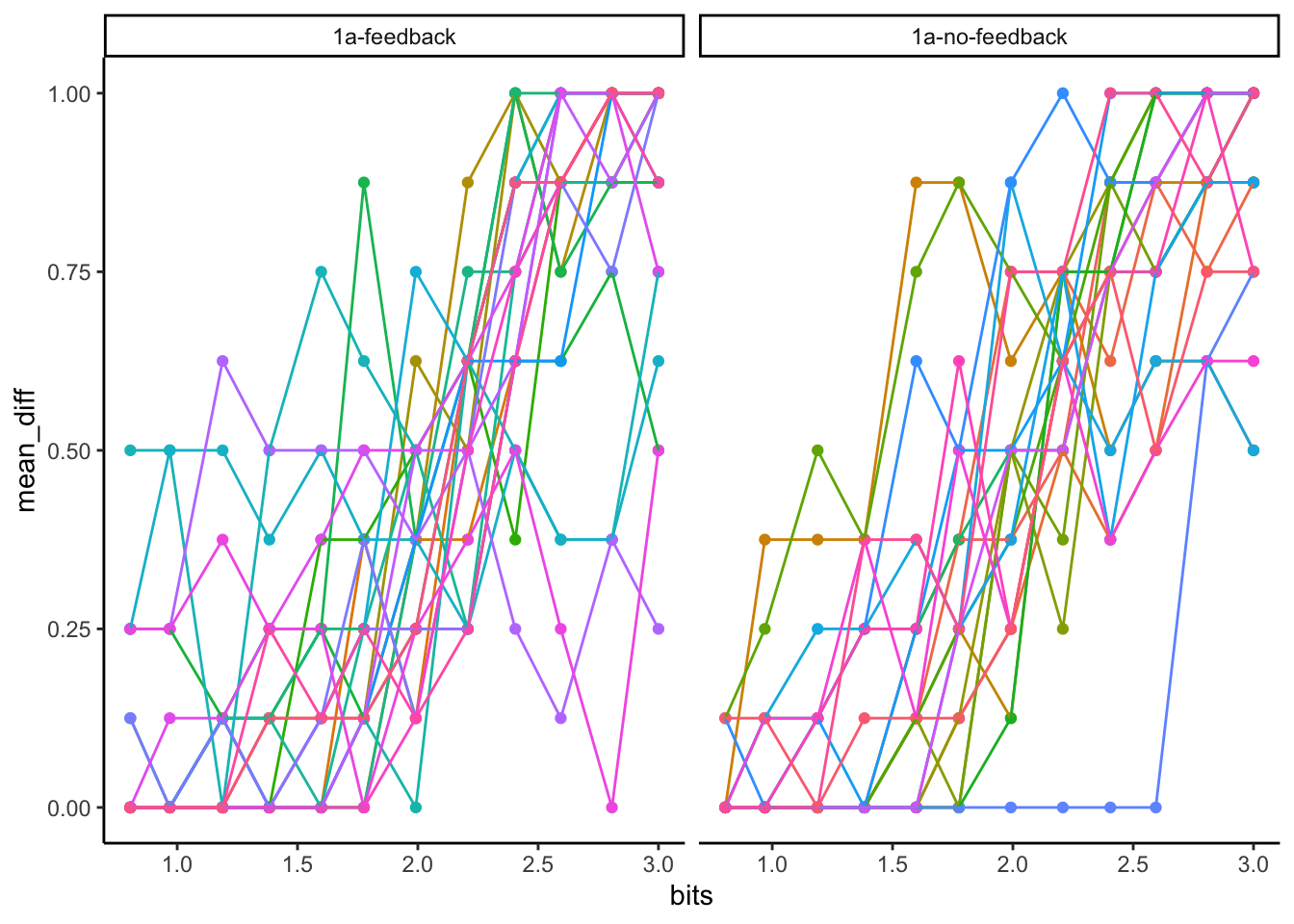

group means

Here we average over the individual subjects.

# average over subjects
group_means <- sub_means %>%
  group_by(counterbalance,bits) %>%
  summarize(mean_diff = mean(mean_diff),.groups = "drop")

#plot
ggplot(group_means, aes(x = bits, y=mean_diff))+
  geom_point()+
  facet_wrap(~counterbalance)+
  theme_classic()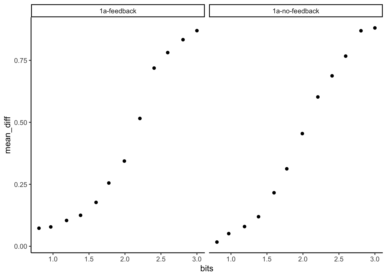

fitting a psychophysics function

library(quickpsy)

# include only rows where a response occurred
filtered_data_psy <- all_data %>%
  filter(task == "judgment")

# format for quickpsy
sub_totals_psy <- filtered_data_psy %>%
  mutate(response = as.numeric(response)) %>%
  group_by(counterbalance,bits) %>%
  summarize(sum_response = sum(response),
            total_response = n(),
            .group = "drop"
            )

#fit curve
try_fit <- quickpsy(sub_totals_psy,
         x = bits,
         k = sum_response,
         n = total_response,
         guess = TRUE,
         grouping = .(counterbalance))
# plot
plotcurves(try_fit)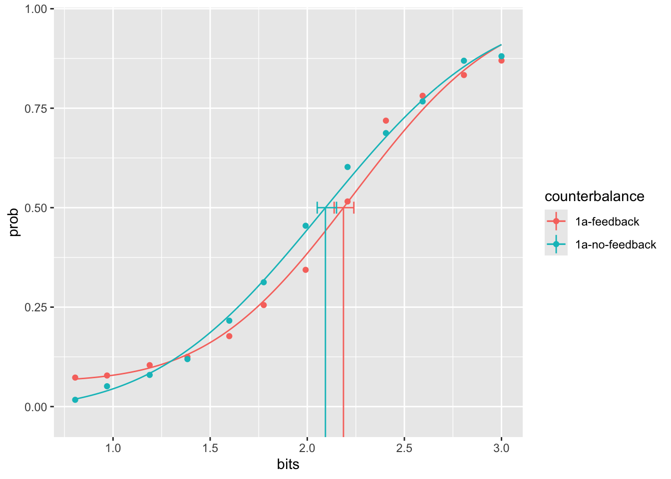

# print parameters
try_fit$par

# A tibble: 6 × 5
# Groups:   counterbalance [2]
  counterbalance parn      par  parinf parsup
  <chr>          <chr>   <dbl>   <dbl>  <dbl>
1 1a-feedback    p1     2.24    2.17   2.30  
2 1a-feedback    p2     0.587   0.521  0.664 
3 1a-feedback    p3     0.0623  0.0288 0.0908
4 1a-no-feedback p1     2.08    2.02   2.15  
5 1a-no-feedback p2     0.680   0.599  0.755 
6 1a-no-feedback p3    -0.0116 -0.0430 0.0216

save workspace

save.image("data/1a_analysis.RData")

Using inline code to write results.

Inline code snippets allow one to write R results within a text segment. This is an R code snippet that prints the value of 1+1 = 2. We can use R code snippets to write results.

Psychophysical functions were fit to the data in each feedback condition using cumulative normal curves. The point of subject equality in the feedback condition was 2.19. Note this value was read in from an R variable and printed here. We will use this style of reporting in the main manuscript to make sure our results are reproducible.

Pilot cluster analysis

load("data/Sequence_matrix.RData")

# function to compute mean inter-item distance
mean_item_distance <- function(x){
  
  x_to_char <- as.character(x)
  all_unique <-  unique(x_to_char)
  counter <- rep(0,length(all_unique))
  names(counter) <- all_unique
  
  all_differences <- c()
  for(i in 1:length(all_unique)){
    differences <- diff( which(x_to_char %in% all_unique[i]  == TRUE), diff = 1)
    differences <- c(0,(differences-1))
    all_differences <- c(all_differences,differences)
  }

  return(mean(all_differences))
  
}

clustering_scores <- apply(sequences_matrix,MARGIN = 1,mean_item_distance)

cluster_df <- data.frame(file_name = names(clustering_scores),
                         clustering = clustering_scores)

new_filtered <- filtered_data %>%
  mutate(file_name = gsub("mp3s/","", stimulus)) %>%
  mutate(file_name = gsub(".mp3",".mid",file_name)) %>%
  mutate(response = as.numeric(response))

new_filtered <- left_join(new_filtered,cluster_df,'file_name')

ggplot(new_filtered, aes(x=clustering,y=response))+
  geom_point()+
  geom_smooth(method = "lm")+
  facet_wrap(~bits, scales = "free")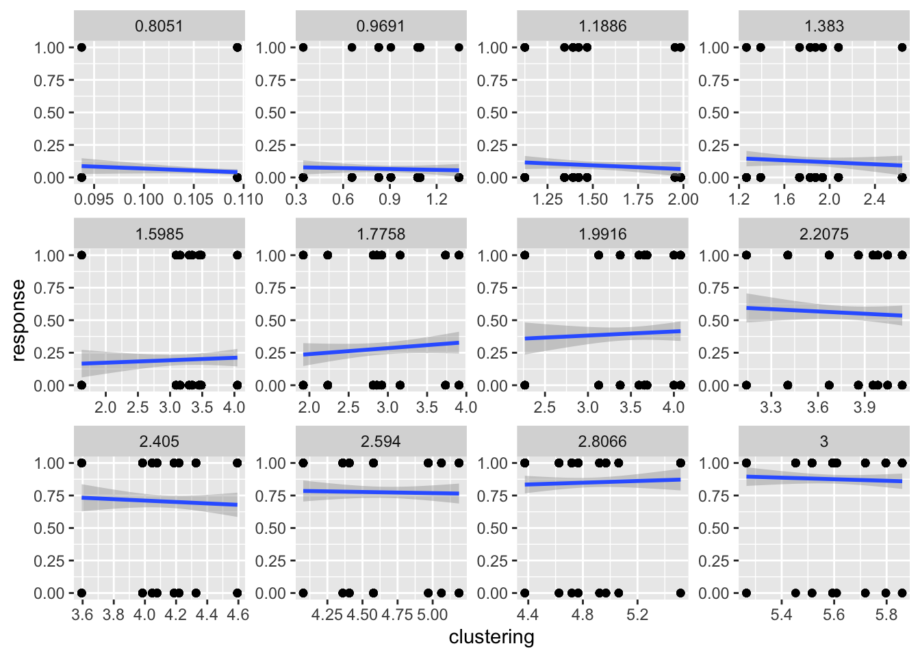

plot(new_filtered$bits,new_filtered$clustering)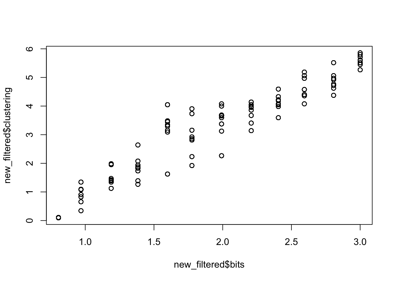

sort(unique(new_filtered$bits))

 [1] 0.8051 0.9691 1.1886 1.3830 1.5985 1.7758 1.9916 2.2075 2.4050 2.5940
[11] 2.8066 3.0000