Lab 6 Statistical Inference

Readings and Review

This lab marks a departure into the land of statistical inference. We have been working toward these concepts and using R to help us understand basic aspects of distributions and sampling from distributions. These concepts will be applied throughout the remainder of the course as we discuss many different tools and tests and for statistical inference.

As your instructor (Matt Crump), you should know that I have many “feelings” about statistical inference. That is, I have many perspectives, sometimes competing and even inconsistent ones, about the value, goals, and practice of “doing statistical inference”. This is partly because there are many well-founded opinions and approaches to statistical inference out there to try out, and also partly because there are many known issues and flawed practices that researchers sometimes engage in, and there also many limitations to the kinds of inferences that can be made depending on what you are doing.

To take one example, a researcher might want to do an “X test” on their data, and even though they don’t really know what the “X test” is all about, they know that they can put their data into a program and press a button, and the program will do the X test, and then they can report the results of the X test in a paper. My view is that this kind of behavior is irresponsible. My view is that, in general, the researcher should have extremely well thought out reasons and justifications and motivations in advance of collecting the data for how they will do the analysis. They should be able to describe how the X test works, what it’s assumptions are, and why it is appropriate to use in their case, as well as what it’s limitations are, and what exactly can be concluded from the test.

Another example is more in line with my view. A researcher understands the general principles of how statistical inference works, they collect data in a particular experiment that they designed, and they make up and use their own custom test that is completely justifiable for the issue they are addressing.

Be able to justify your statistical inference

Both of these examples are kind of extreme cases. However, whether you use a well-known test, a common canned approach, or roll-your-own statistics, I strongly believe that you should be able to justify your approach. This means you will be able to present an argument about why your process for statistical inference is minimally suitable for the task at hand.

And, because I think being able to justify your statistical inferences is so important, I have designed the following labs to help you learn about fundamental principles of statistical inference, so you can use them to understand and justify and even create your own process of statistical inference that is appropriate to the research you are doing.

Foundations for Statistical Inference and the Crump test

If you are new to the concept of tests for statistical inference, and/or if you want a slightly unconventional take on statistical inference, I’ll forward you to a chapter from my undergraduate statistics textbook: https://crumplab.github.io/statistics/foundations-for-inference.html. This chapter discusses some basic ideas behind statistical inference, and it also provides a test that I “made up” called the Crump test, which doesn’t use any formulas, and tries to highlight the process and ideas behind statistical inference.

A parting metaphor

Imagine you are a detective at the scene of a crime. You want to know who committed the crime. Another detective says, I have a hypothesis, the crime scene is consistent with how I believe Mickey Mouse would have committed the crime. You are puzzled, after all Mickey Mouse is a fictional cartoon character, it is impossible that Mickey Mouse committed the crime. You ask for clarification. The other Detective says, “I mean that, IF Mickey Mouse was real, I think he could have committed the crime”. Also, several other detectives say that they do not think Donald Duck did it, by which they mean, the crime scene is inconsistent with how Donald Duck would have done the crime IF Donald Duck was real.

You might be wondering what I am on about with this metaphor? I would imagine the detective finds it strange to even consider hypotheses about how fictional cartoon characters may or may not have committed a crime. In my view, this strangeness is not too different from how a researcher considers statistical hypotheses about the data they collect. As we will see throughout the rest of the course, the statistical hypotheses sometimes are not too different from fictional characters, and although they can be immensely useful for some tasks of data analysis and interpretation, they are not without clear limitations in their explanatory power.

Overview

We begin our discussion of statistical tests with Permutation and Randomization tests.

Concepts I: Permutation test
Concepts II: Randomization test
Practical I: Randomization test on real data

Why are these tests not very common?

If you have read many research papers in psychology, you might not see very many permutation or randomization tests being reported. Specific disciplines and sub-disciplines tend to adopt specific tests for various reasons, and inertia can set in. If the tests that are being used are good enough, why use different ones?

Permutation and randomization tests are good examples of tests that are “easy” for a computer to do, and “hard” for a person to do. This is because conducting the process of permuting and/or random sampling by hand can take a very long time. The manual labor involved is probably one reason why these tests did not become popular before computers were invented. And, because the use of specific other tests in the discipline was already firmly established before computers were widely available, it seems that these permutation and randomization tests fell by the wayside. If computers were available earlier on, my guess is that these test would be used more commonly today.

Fortunately, we have computers and R, so we can now use them to create and evaluate our own permutation and randomization tests.

C1: Permutation Test

What is a permutation?

A permutation is a reordering of a sequence. For example, we can easily re-order the sequence in a by using the sample() function.

a <- c(1,2,3,4,5)
sample(a)
#> [1] 4 2 5 1 3

The number of permutations (unique re-orderings) for n distinct items is \(n!\)

Therefore, if we take 5 numbers from the distinct values 1, 2, 3, 4, 5, we will be able to form 120 distinct orders or permutations of those numbers.

5*4*3*2*1
#> [1] 120

If you were to put the numbers 1, 2, 3, 4, 5 into a basket, and randomly take them out, what are the chances you take them out in the order 1,2,3,4,5?

Well, that is 1 order out of 120, so 1/120 =

1/120
#> [1] 0.008333333

Let’s quickly test this:

# generate 10000 random samples
my_samples <- replicate(10000,sample(c(1,2,3,4,5)))

count_examples <- 0 
for(i in 1:10000){
  if( sum( my_samples[,i] == c(1,2,3,4,5) ) == 5) {
    count_examples <- count_examples+1
  } 
}

count_examples/10000
#> [1] 0.0076

A quick summary. Permutations are different ways to order numbers. For a given set of numbers, there is always a total number of possible orders. If we assume that any of the orders could have been obtained by chance, then we can calculate the chances of getting a particular order.

A permutation test example

There are 8 people, and you assign 4 to group A, and 4 to group B. You have a basket that contains 8 balls, each with a number on it, just like a lottery. The balls are numbered from 1 to 8, and are completely identical. Everybody puts on a blindfold and goes up one at a time to take one ball.

What are the possible outcomes in this situation? First, there are \(8! = 8*7*6*5*4*3*2*1 = 40,320\) possible permutations, which is the number of different ways that each person from each group could randomly choose a ball.

This also means that the chances of getting a highly specific outcome, like below is is \(1/40320\), or 2.4801587^{-5}.

example_outcome <- data.frame(group = rep(c("A","B"),each=4),
                              person = c(1,2,3,4,1,2,3,4),
                              ball = sample(1:8)
)
knitr::kable(example_outcome)

group	person	ball
A	1	8
A	2	7
A	3	3
A	4	5
B	1	2
B	2	4
B	3	1
B	4	6

What are the chances that sum of the balls in Group A will be very different from the sum of the balls chosen by Group B? We could figure these kinds of questions out if we had access to all of the permutations. Let’s make a matrix of all of the possible permutations.

First, install the package ‘combinat’, which contains the permn() function. We can use this function to create matrix of all permutations of the sequence 1 to 8. Note, if your sequence is much larger, the number of permutations becomes very very large, so I wouldn’t recommend using this function to generate permutations for very large sequences.

library(combinat)
#> 
#> Attaching package: 'combinat'
#> The following object is masked from 'package:utils':
#> 
#>     combn
permutation_matrix <- matrix(unlist(permn(1:8)), ncol=8, byrow=TRUE)

In this matrix we can assume that the first four columns are the choices that persons 1 to 4 in group A could have made, and the last four columns are the choices that persons 5 to 8 could have made.

Let’s now determine the various sums that could be obtained for each permutation. That is, if we sum up the ball numbers for Group A and group B, we can learn what all of the different possible outcomes actually are.

group_A_sums <- rowSums(permutation_matrix[,1:4])
group_B_sums <- rowSums(permutation_matrix[,5:8])

Now, let’s determine all of the possible differences between the sums for Group A and B.

possible_differences <- group_A_sums - group_B_sums

What do these possible differences look like? Let’s make a histogram.

hist(possible_differences)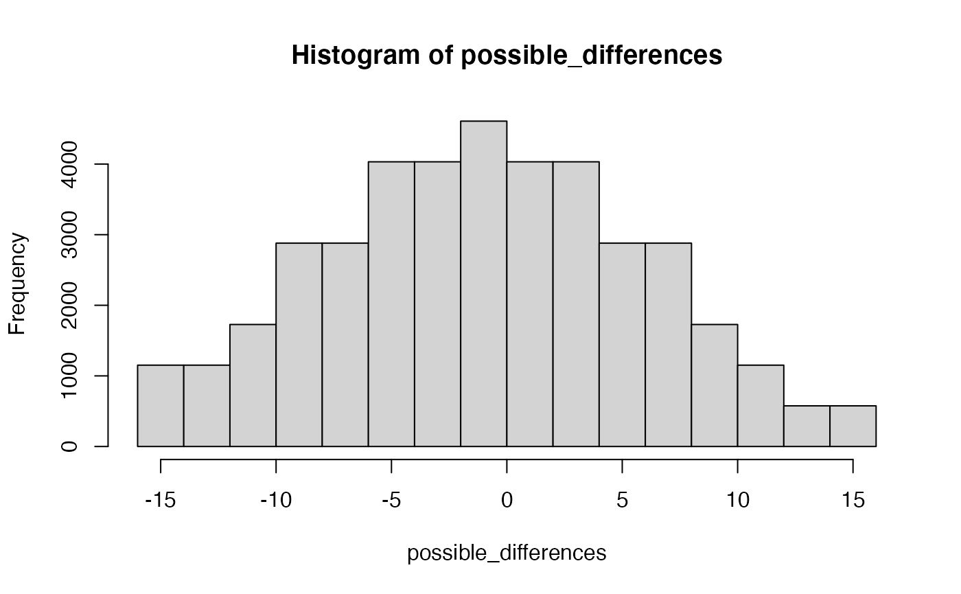

Let’s do a sanity check. What is the biggest possible difference that could be obtained? That would occur if one group chose the 4 smallest numbers (1,2,3,4), which sums to 10; and the other group chose the 4 biggest numbers (5,6,7,8), which sums to 26. Therefore, the largest possible difference is 26-10 = 16.

What is the largest difference observed in our possible_differences vector? Checks out, that’s good.

max(possible_differences)
#> [1] 16

Let’s now answer some specific questions. What is the probability that the difference in the group sums will be larger than 16? Because we have just determined that this is impossible, we can confidently say 0.

possible_differences[possible_differences > 16]
#> numeric(0)

What is the probability that the absolute value of the difference in the group sums will be larger than 10?

First, we convert all of the differences to positive values:

absolute_differences <- abs(possible_differences)

Then we figure out how many differences are larger than 10, and divide by the total possible outcomes:

length(absolute_differences[absolute_differences > 10])/length(absolute_differences)
#> [1] 0.1142857

Interim Summary: General Principles

In a permutation test we:

obtain data in different conditions
permute the data across conditions to produce all possible outcomes, or ways that the data could have been obtained across the conditions
Calculate the odds that specific data patterns (a subset of permutations) could have occurred relative to all of the possible permutations.

More generally, we obtain data which is a specific case example. This is “what did happen”. We are interested in “what could have happened”, so we generate all the possible outcomes. Then we compare some summary of what did happen, to what could have happened. What do we learn from this exercise? In our current example, we learn about how chance can produce differences of various sizes.

Permutation test on experimental data.

Consider an experiment was conducted that had two groups A and B. There were 8 total participants, and they were randomly assigned to the groups. Group A received 1 million dollars as motivation to do well on a midterm. Group B received 0 dollars. Both groups took a midterm. The mean performance for each subject in group A was 85, 75, 76, and 89. The mean performance for each subject in Group B was 90, 65, 68, 69.

group_A <- c(85,75,76,89)
group_B <- c(90,65,68,69)

Overall the mean for group A was:

mean(group_A)
#> [1] 81.25

And, the mean for group B was:

mean(group_B)
#> [1] 73

So, group A, who got a million dollars, on average did better on the midterm than group B. The difference was 81.25 - 73 = 8.25.

mean(group_A) - mean(group_B)
#> [1] 8.25

What caused the difference?

Did the experimental manipulation cause the difference? Did giving group A one million dollars cause them to somehow do better on the test? We could consider this as one possibility.

Are there other possibilities? What other kind of process could have caused the pattern of numbers that we observed? Another possible explanation is random sampling, which is how we assigned participants to the groups. It is possible that group A randomly had more participants that were more prepared for the test.

Assessing chance with a permutation test

We can use a permutation test to assess all of the possible ways that participants and their scores could have been assigned to groups. Then we can calculate all of the possible group differences that could have been observed. Then we can compare the group difference that we did observe (8.25), to the group differences that we could have observed. This will let us know if the random sampling process was likely or unlikely to produce the difference.

# put all means in a variable
all_scores <- c(group_A,group_B) 

# generate permutation matrix
permutation_matrix <- matrix(unlist(permn(all_scores)), ncol=8, byrow=TRUE)

# calculate overall group means for each permutation
group_A_means <- rowSums(permutation_matrix[,1:4])/4
group_B_means <- rowSums(permutation_matrix[,5:8])/4

# generate all possible differences
possible_differences <- group_A_means - group_B_means

The possible_differences vector contains all of the possible mean differences that could have been produced by random sampling. Let’s compare this to what we observed. We will do this in two ways.

# visualize the analysis

library(ggplot2)

qplot(possible_differences)+
  geom_histogram(color="orange")+
  geom_vline(xintercept=mean(group_A) - mean(group_B), color ="red")+
  theme_classic()
#> `stat_bin()` using `bins = 30`. Pick better value with `binwidth`.
#> `stat_bin()` using `bins = 30`. Pick better value with `binwidth`.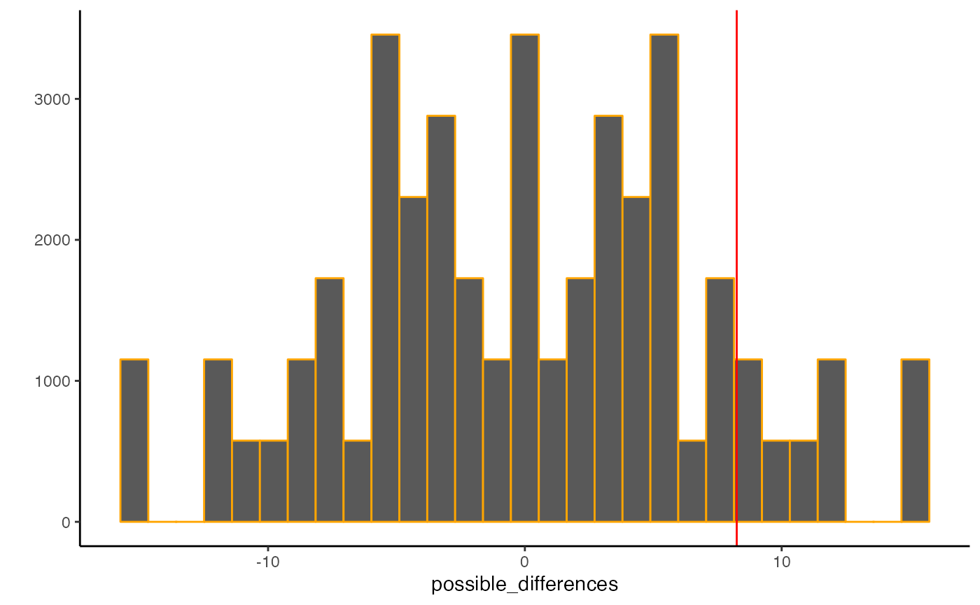

The histogram shows all of the possible differences we could have obtained by randomly sampling the participants into the different groups. The red line shows the difference that was obtained. These are all facts of this example.

I like to the think of the “distribution of possible differences” as a window of opportunity for chance. That is, we are looking at differences in the data that could have been produced by chance. We also see that some values occur more often than others. For example, the red line, with the observed difference of 8.25 is 1) inside the distribution, which means that chance could have produced this difference, but 2) it is kind of far to the left, so it seems that chance doesn’t produce a difference this big very often.

We could be more precise and calculate the odds of getting a difference of 8.25 or larger, which I find to be 11.4%.

length(possible_differences[possible_differences >= 8.25]) / length(possible_differences)
#> [1] 0.1142857

So…to return the cartoon character metaphor, we have a who dunnit question. Was Mickey Mouse with the million dollars that caused the difference of 8.25? Or was it Donald Duck with random chance that accidentally produced a difference of 8.25? We know that Mr. Duck only produces a difference of 8.25 or larger 10% of the time…Is that enough to say that Mr. Duck DID NOT DO IT? I don’t think so. He clearly could have done it. Can we be absolutely certain that it was the million dollar manipulation? No. Have we learned anything useful at all? I think so, it seems we got a result that is irregular from the perspective of chance. This might give me some confidence that the experimental manipulation actually caused the difference, and not the act of randomly assigning participants to groups.

If it was just chance, then I would expect that this experiment wouldn’t replicate, and that on average there wouldn’t be big differences between groups. On the other hand, if the replications showed a big difference over and over again, I would be more confident the manipulation caused the difference.

C2: Randomization test

The randomization test is a version of the permutation test that can be used when the number of permutations is very large and impractical to generate. For example, in the previous toy example we only had 8 means, and permuting them across two groups required generating 40320 sequences. If you had hundreds or thousands of subjects, your computer would quickly loose the memory capacity to generate all of the possible permutations. Instead, we randomly sample from the possible permutations, and create a sampling distribution, and use this to become informed about what could have happened by chance.

Imagine you had 50 subjects each in group A and B. Let’s generate fake scores for each participant. Let’s also imagine that in this experiment the manipulation actually DOES NOT WORK. So, we will pretend that the scores for each participant are coming from the very same distribution, let’s say a normal distribution with mean = 65 and sd = 10.

group_A <- rnorm(50,65,10)
group_B <- rnorm(50,65,10)

We can then calculate the mean of each group, and look at the difference.

mean(group_A)
#> [1] 65.29572
mean(group_B)
#> [1] 66.51585
mean(group_A)-mean(group_B)
#> [1] -1.220125

In some general sense if the manipulation works, that is it causes a difference, then we would expect to see a non-zero difference. If the manipulation is ineffective and does nothing, then we expect on average no difference, however we recognize that we could obtain differences just by chance alone, because of randomly sampling our participants into the different groups.

We now want to calculate a sampling distribution of possible mean differences. To do this, we take all of the values in Group A and B, and randomly re-assign them across both groups, then recalculate the means and the mean difference. Then we, do this multiple times, as in monte-carlo simulation.

# creating one random permutation
all_scores <- c(group_A,group_B)
resample <- sample(all_scores)
new_A_mean <- mean(resample[1:50])
new_B_mean <- mean(resample[51:100])
new_difference <- new_A_mean-new_B_mean
new_difference
#> [1] -3.575433

# Simulate the above process 10000 times
mean_differences <- c()
for(i in 1:10000){
  resample <- sample(all_scores)
  new_A_mean <- mean(resample[1:50])
  new_B_mean <- mean(resample[51:100])
  mean_differences[i] <- new_A_mean-new_B_mean
}

Now we can plot the mean differences to get a sense of the kinds of differences that chance could have produced, again the red line shows a particular mean difference that was observed in this toy example.

qplot(mean_differences)+
  geom_histogram(color="orange")+
  geom_vline(xintercept=mean(group_A) - mean(group_B), color ="red")+
  theme_classic()
#> `stat_bin()` using `bins = 30`. Pick better value with `binwidth`.
#> `stat_bin()` using `bins = 30`. Pick better value with `binwidth`.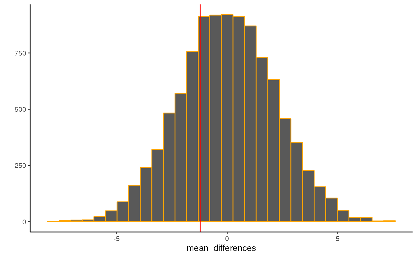

The above histogram is a “sampling distribution of mean differences”, and it shows the kinds of differences between group A and group B that could be obtained purely because of randomly assigning people to different groups.

In terms of a detective novel, this is chances alibi, it shows what chance is capable of doing. In this situation, chance alone could easily produce differences between group A and B as large as 4 or -4. Notice, that chance never produces a difference as large as 20. If you had all the information that we have in this example, then as a researcher you could attempt to rule out the possibility that was chance was involved in producing a difference that you observed.

We can also use this distribution to calculate specific probabilities concerning chance. For example, what is the probability of getting a 4 or larger by chance alone?

length(mean_differences[mean_differences >=4 ])/length(mean_differences)
#> [1] 0.0327

P1: Randomization test with real data

Randomization tests are very flexible and can be constructed for most experiments. They simply involve:

randomizing all of the data across the conditions
calculating a statistic of interest
Do the above thousands of times to create a sampling distribution for the statistic of interest
Compare the observed statistic of interest (e.g., a difference between group means) to the sampling distribution to determine if the observed statistic was A) likely to have been produced by random sampling, or B) unlikely to be produced by random sampling

Here I construct a randomization test for an experiment asking the question…Do you come across as smarter (in an interview) when evaluators get to hear what you say, or only get to read what you say.

You can learn more about the experiment here: https://crumplab.github.io/statisticsLab/lab-7-t-test-independent-sample.html. This is a link to a lab manual that gives an example of conducting a t-test, something we will discuss in later labs. We will use the data from this experiment, which is contained in your ‘open_data’ folder, and titled, SchroederEpley2015data.csv, and we will conduct a randomization test.

Note that the condition code 1 refers to the audio group, and 0 refers to the reading only group.

#load the data
the_data <- read.csv("open_data/SchroederEpley2015data.csv", header = TRUE)

# compute the group means
library(dplyr)
#> 
#> Attaching package: 'dplyr'
#> The following objects are masked from 'package:stats':
#> 
#>     filter, lag
#> The following objects are masked from 'package:base':
#> 
#>     intersect, setdiff, setequal, union

the_data %>% 
  group_by(CONDITION) %>%
  summarize(group_means = mean(Intellect_Rating))
#> # A tibble: 2 × 2
#>   CONDITION group_means
#>       <int>       <dbl>
#> 1         0        3.65
#> 2         1        5.63

We can see that the audio only group (1) received higher intellect ratings (5.63) than the read only group (0), 3.64. The difference, or effect was about 2.

Was this difference a result that could have occurred because of randomly assigning people to different groups? Let’s do a randomization test to create a sampling distribution of possible mean differences.

# restrict the dataset to the columns of interest
simulation_data <- the_data %>%
  select(CONDITION,Intellect_Rating)

# example of randomizing the scores across conditions
simulation_data %>%
  mutate(Intellect_Rating = sample(Intellect_Rating))
#>    CONDITION Intellect_Rating
#> 1          1        3.3333333
#> 2          1        1.6666667
#> 3          1        7.6666667
#> 4          0        9.0000000
#> 5          0        6.0000000
#> 6          0        1.6666667
#> 7          1        3.6666667
#> 8          0        0.6666667
#> 9          1        2.0000000
#> 10         0        1.0000000
#> 11         0        4.6666667
#> 12         1        2.3333333
#> 13         1        5.0000000
#> 14         0        4.6666667
#> 15         0        5.6666667
#> 16         1        7.0000000
#> 17         1        3.6666667
#> 18         1        6.0000000
#> 19         0        6.0000000
#> 20         0        5.3333333
#> 21         0        6.6666667
#> 22         0        5.0000000
#> 23         0        3.3333333
#> 24         1        3.3333333
#> 25         1        6.6666667
#> 26         1        5.0000000
#> 27         0        3.6666667
#> 28         1        4.6666667
#> 29         1        6.3333333
#> 30         1        4.6666667
#> 31         0        2.3333333
#> 32         0        9.0000000
#> 33         1        5.6666667
#> 34         1        5.6666667
#> 35         0        3.6666667
#> 36         1        5.6666667
#> 37         0        6.0000000
#> 38         1        6.0000000
#> 39         1        3.6666667

# example of calculating a new mean difference

new_data <- simulation_data %>%
  mutate(Intellect_Rating = sample(Intellect_Rating)) %>%
  group_by(CONDITION) %>%
  summarize(new_means = mean(Intellect_Rating), .groups="drop")

new_data
#> # A tibble: 2 × 2
#>   CONDITION new_means
#>       <int>     <dbl>
#> 1         0      4.61
#> 2         1      4.81
new_data[new_data$CONDITION == 0,]$new_means
#> [1] 4.611111
new_data[new_data$CONDITION == 1,]$new_means
#> [1] 4.809524
new_difference <- new_data[new_data$CONDITION == 1,]$new_means-new_data[new_data$CONDITION == 0,]$new_means

# Run a randomization test

possible_differences <-c()
for(i in 1:1000){
  # permute the data and calculate new means
  new_data <- simulation_data %>%
    mutate(Intellect_Rating = sample(Intellect_Rating)) %>%
    group_by(CONDITION) %>%
    summarize(new_means = mean(Intellect_Rating), .groups='drop')
  
  # calculate and save mean difference
  possible_differences[i] <- new_data[new_data$CONDITION == 1,]$new_means-new_data[new_data$CONDITION == 0,]$new_means
}

Now we look the sampling distribution of possible differences, and compare the observed difference of 2, to what could have happened:

qplot(possible_differences)+
  geom_histogram(color="orange")+
  geom_vline(xintercept=2, color ="red")+
  theme_classic()
#> `stat_bin()` using `bins = 30`. Pick better value with `binwidth`.
#> `stat_bin()` using `bins = 30`. Pick better value with `binwidth`.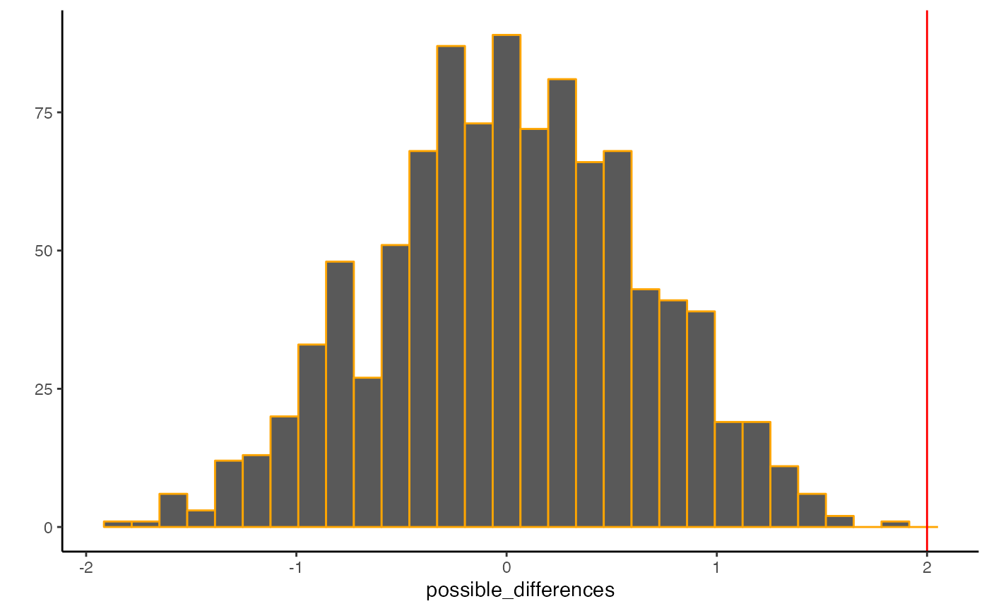

It’s pretty clear in this example that a mean difference of 2 rarely occurred across the random shuffles of the data. The odds of getting 2 or larger from the simulation were:

length(possible_differences[possible_differences >= 2]) / length(possible_differences)
#> [1] 0

What can be concluded from this exercise? Should we conclude that that experimental manipulation actually caused the difference in Intellect ratings? Should we conclude that chance did not produce the difference?

I’m a bit more conservative about what can be concluded. I would say that the exercise of producing the sampling distribution of differences was very useful. It gives me a pretty good sense of the kinds of differences that chance alone could produce. It shows me that a difference of 2 is very rarely produced by chance alone. This gives me some confidence to rule out chance as a candidate. In other words, I do not really think that chance has a great alibi, it wouldn’t have produced the pattern in the data very often. At the same time, it could have, just not very often…so, we can be confident, but not completely sure that chance didn’t do it.

As for the experimental manipulation…if it wasn’t chance that caused the difference, is it necessarily the case that the manipulation caused the difference? This is like saying Donald Duck did not cause the difference, therefore my manipulation did cause the difference. It makes no sense. Instead, sure, the manipulation could have caused the difference, also maybe there were other confounds that were not addressed that caused the difference. Ruling out chance doesn’t tell you what caused the difference, it just suggests that the difference wasn’t caused by chance.

Some coding alternatives

The script for a randomization test could be written in many different ways. Here are is an additional example:

#load the data
the_data <- read.csv("open_data/SchroederEpley2015data.csv", header = TRUE)

# compute the group means
the_data %>% 
  group_by(CONDITION) %>%
  summarize(group_means = mean(Intellect_Rating))
#> # A tibble: 2 × 2
#>   CONDITION group_means
#>       <int>       <dbl>
#> 1         0        3.65
#> 2         1        5.63

# how many participants per group?
table(the_data$CONDITION)
#> 
#>  0  1 
#> 18 21

# create permutations
mean_differences <- c()
for(i in 1:10000){
  resample <- sample(the_data$Intellect_Rating)
  new_1_mean <- mean(resample[1:18])
  new_0_mean <- mean(resample[19:39])
  mean_differences[i] <- new_1_mean-new_0_mean
}

#plot
qplot(mean_differences)+
  geom_histogram(color="orange")+
  geom_vline(xintercept=2, color ="red")+
  theme_classic()
#> `stat_bin()` using `bins = 30`. Pick better value with `binwidth`.
#> `stat_bin()` using `bins = 30`. Pick better value with `binwidth`.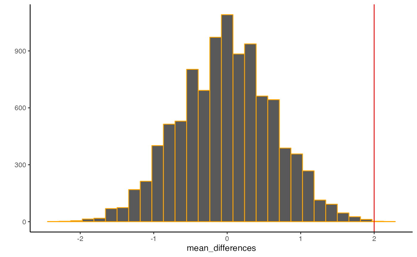

Lab 6 Generalization Assignment

Instructions

In general, labs will present a discussion of problems and issues with example code like above, and then students will be tasked with completing generalization assignments, showing that they can work with the concepts and tools independently.

Your assignment instructions are the following:

Work inside the R project “StatsLab1” you have been using
Create a new R Markdown document called “Lab6.Rmd”
Use Lab6.Rmd to show your work attempting to solve the following generalization problems. Commit your work regularly so that it appears on your Github repository.
For each problem, make a note about how much of the problem you believe you can solve independently without help. For example, if you needed to watch the help video and are unable to solve the problem on your own without copying the answers, then your note would be 0. If you are confident you can complete the problem from scratch completely on your own, your note would be 100. It is OK to have all 0s or 100s anything in between.
Submit your github repository link for Lab 6 on blackboard.
There is one problem to solve

Problems

Write a function that conducts a randomization test for the mean difference between two groups, and show that it works. Specifically, using your function, conduct a randomization test on the same data we used in the above example from lab. Report the results and briefly discuss what the results of the randomization tell you. (6 points). Extra: if the observed mean difference in the experiment was found to be .5, what would you have concluded from the randomization test?

Inputs:

the inputs should include a vector for group 1, and vector for group 2, and the number of permutations/re-samplings of the data to create.

Outputs:

output each group mean, and the difference between group means
output a histogram of the sampling distribution of the possible mean differences produced by the randomization process
output the probability or odds of obtaining the observed mean difference or larger.

Optional:

include the ability to calculate the probability of obtaining any mean difference or larger
deal with negative difference scores appropriately
add one or two-tailed test options

Matthew J. C. Crump

10/8/2020