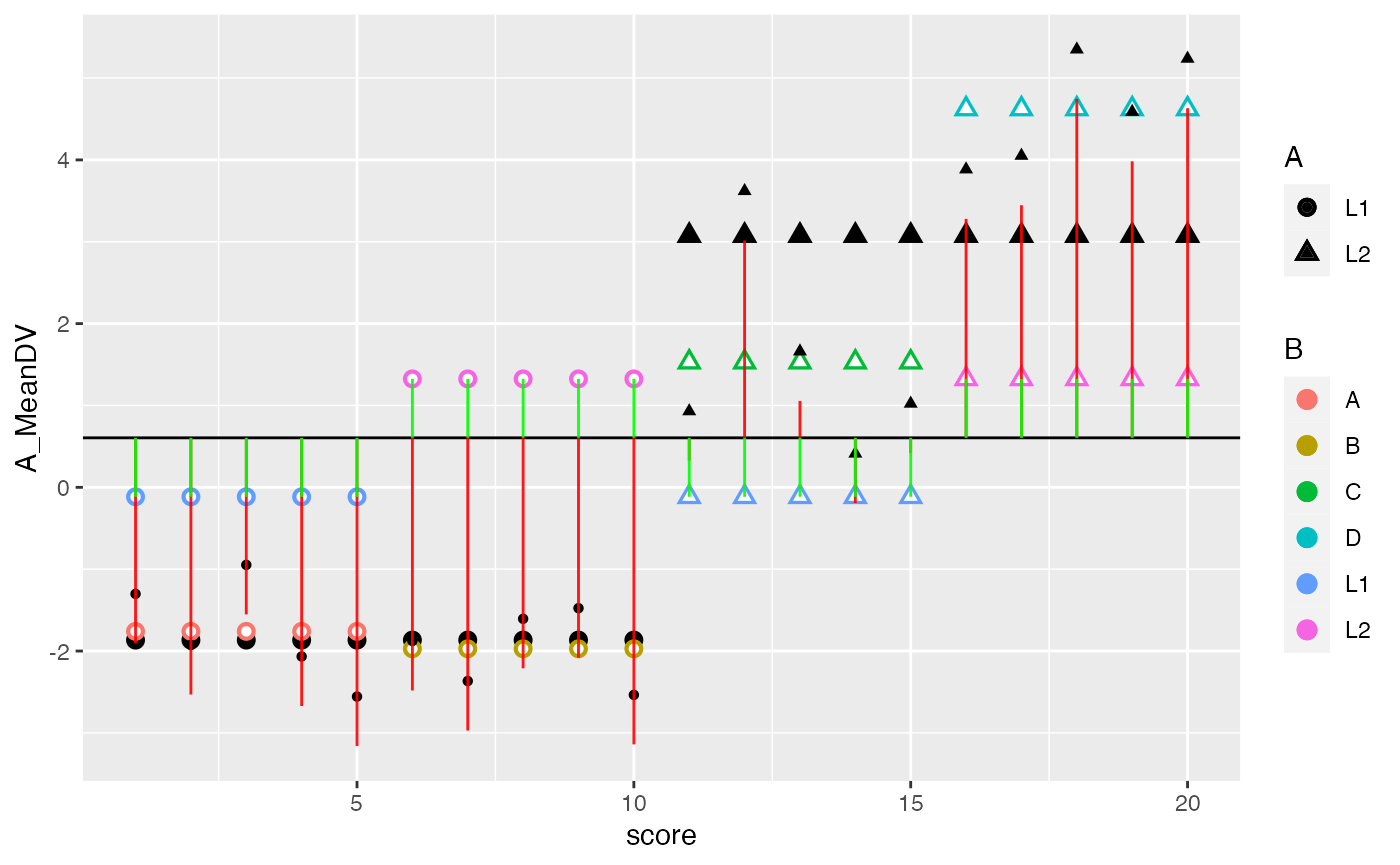
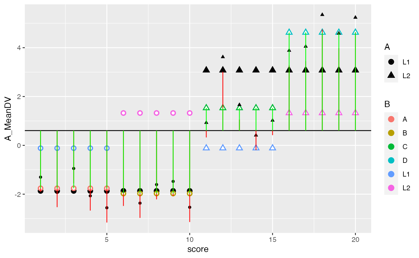
- Explain the concept of main effects and interactions with an example using R. For example, this could include a definition of main effects and interactions and a figure depicting main effects and an interaction along with an explanation of the patterns for each. A major point of this problem is for you to to engage in the task of developing an explanation of these concepts that would 1) be helpful for you to understand the concepts, and 2) could be helpful for others to understand these concepts. (3 points)
library(tidyverse)
#> ── �[1mAttaching packages�[22m ─────────────────────────────────────── tidyverse 1.3.1 ──
#> �[32m✓�[39m �[34mggplot2�[39m 3.3.5 �[32m✓�[39m �[34mpurrr �[39m 0.3.4
#> �[32m✓�[39m �[34mtibble �[39m 3.1.6 �[32m✓�[39m �[34mdplyr �[39m 1.0.8
#> �[32m✓�[39m �[34mtidyr �[39m 1.2.0 �[32m✓�[39m �[34mstringr�[39m 1.4.0
#> �[32m✓�[39m �[34mreadr �[39m 2.1.2 �[32m✓�[39m �[34mforcats�[39m 0.5.1
#> Warning: package 'tidyr' was built under R version 4.1.2
#> Warning: package 'readr' was built under R version 4.1.2
#> Warning: package 'dplyr' was built under R version 4.1.2
#> ── �[1mConflicts�[22m ────────────────────────────────────────── tidyverse_conflicts() ──
#> �[31mx�[39m �[34mdplyr�[39m::�[32mfilter()�[39m masks �[34mstats�[39m::filter()
#> �[31mx�[39m �[34mdplyr�[39m::�[32mlag()�[39m masks �[34mstats�[39m::lag()
n <- 10
factorial_data <- tibble(A = factor(rep(c("L1","L2"), each = n)),
B = factor(rep(rep(c("L1","L2"), each=n/2),2)),
C = factor(rep(c("A","B","C","D"), each = n/2)),
DV = c(rnorm(n/2,-2,1),
rnorm(n/2,-2,1),
rnorm(n/2,2,1),
rnorm(n/2,4,1))
)
A_means <- factorial_data %>%
group_by(A) %>%
summarise(mean_DV_A = mean(DV))
B_means <- factorial_data %>%
group_by(B) %>%
summarise(mean_DV_B = mean(DV))
cell_means <- factorial_data %>%
group_by(A,B) %>%
summarise(mean_DV_cell = mean(DV))
#> �[1m�[22m`summarise()` has grouped output by 'A'. You can override using the `.groups`
#> argument.
grand_mean <- mean(factorial_data$DV)
factorial_data <- factorial_data %>%
mutate(A_MeanDV = rep(A_means$mean_DV_A, each = n),
B_MeanDV = rep(rep(B_means$mean_DV_B, each = n/2),2),
cell_MeanDV = rep(cell_means$mean_DV_cell, each = n/2),
grand_mean
) %>%
mutate(DV_deviations = DV-grand_mean,
A_deviations = (A_MeanDV - grand_mean),
B_deviations = (B_MeanDV - grand_mean),
straight_cell_deviations = (cell_MeanDV - grand_mean),
cell_deviations = (A_MeanDV-grand_mean) + (B_MeanDV-grand_mean) - (cell_MeanDV-grand_mean)
)
summary(aov(DV~A*B, data=factorial_data))
#> Df Sum Sq Mean Sq F value Pr(>F)
#> A 1 122.09 122.09 185.74 3.19e-10 ***
#> B 1 10.37 10.37 15.78 0.001095 **
#> A:B 1 13.66 13.66 20.78 0.000322 ***
#> Residuals 16 10.52 0.66
#> ---
#> Signif. codes: 0 '***' 0.001 '**' 0.01 '*' 0.05 '.' 0.1 ' ' 1
sum(factorial_data$A_deviations^2)
#> [1] 122.0947
sum(factorial_data$B_deviations^2)
#> [1] 10.36959
sum(factorial_data$straight_cell_deviations^2) # note these are incorrect
#> [1] 146.1229
sum(factorial_data$cell_deviations^2)
#> [1] 13.65857
sum(factorial_data$DV_deviations^2)
#> [1] 156.6404
factorial_data <- factorial_data %>%
mutate(score = 1:(n*2))
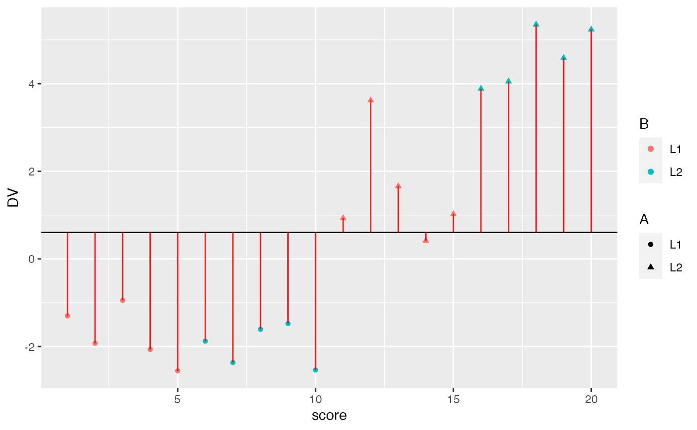
ggplot(factorial_data, aes(x=score, shape=A, color=B))+
geom_hline(yintercept = mean(factorial_data$DV))+
geom_point(aes(y=DV))+
geom_segment(aes(xend = score, y=grand_mean, yend = DV), alpha = .9, color="red")
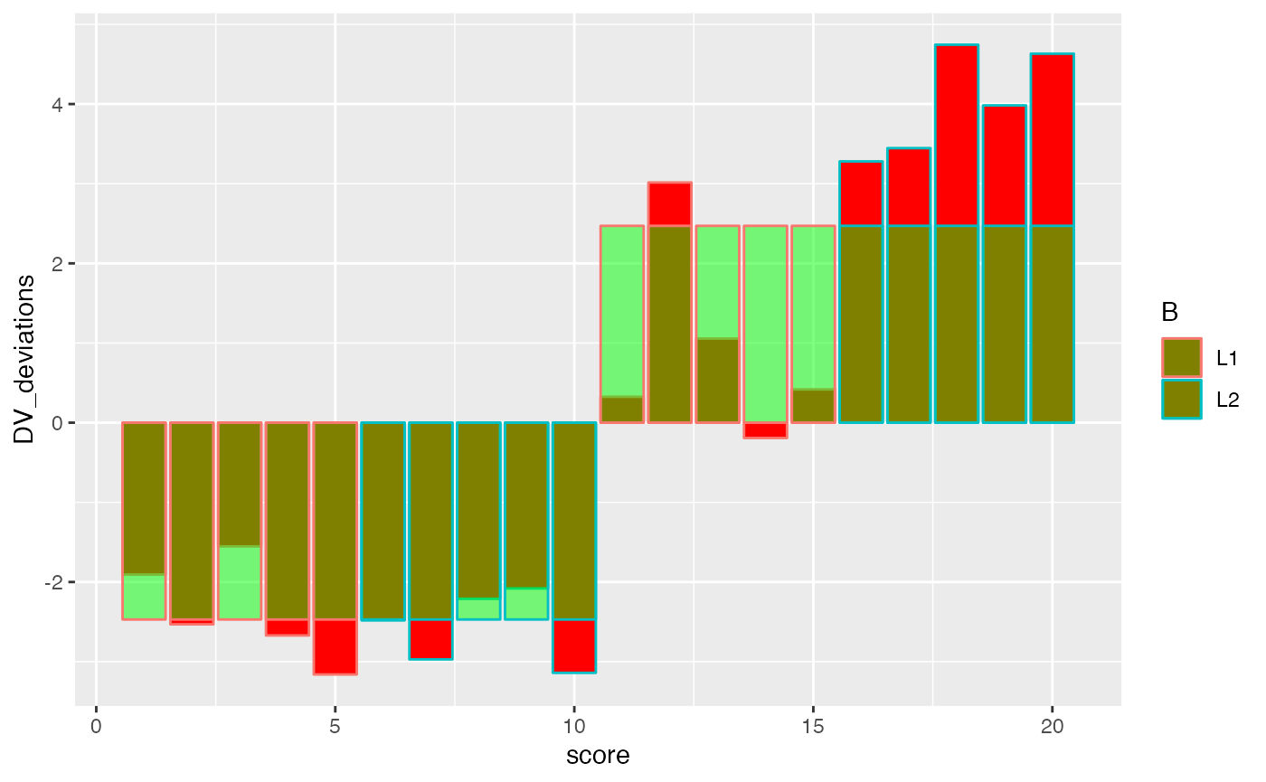
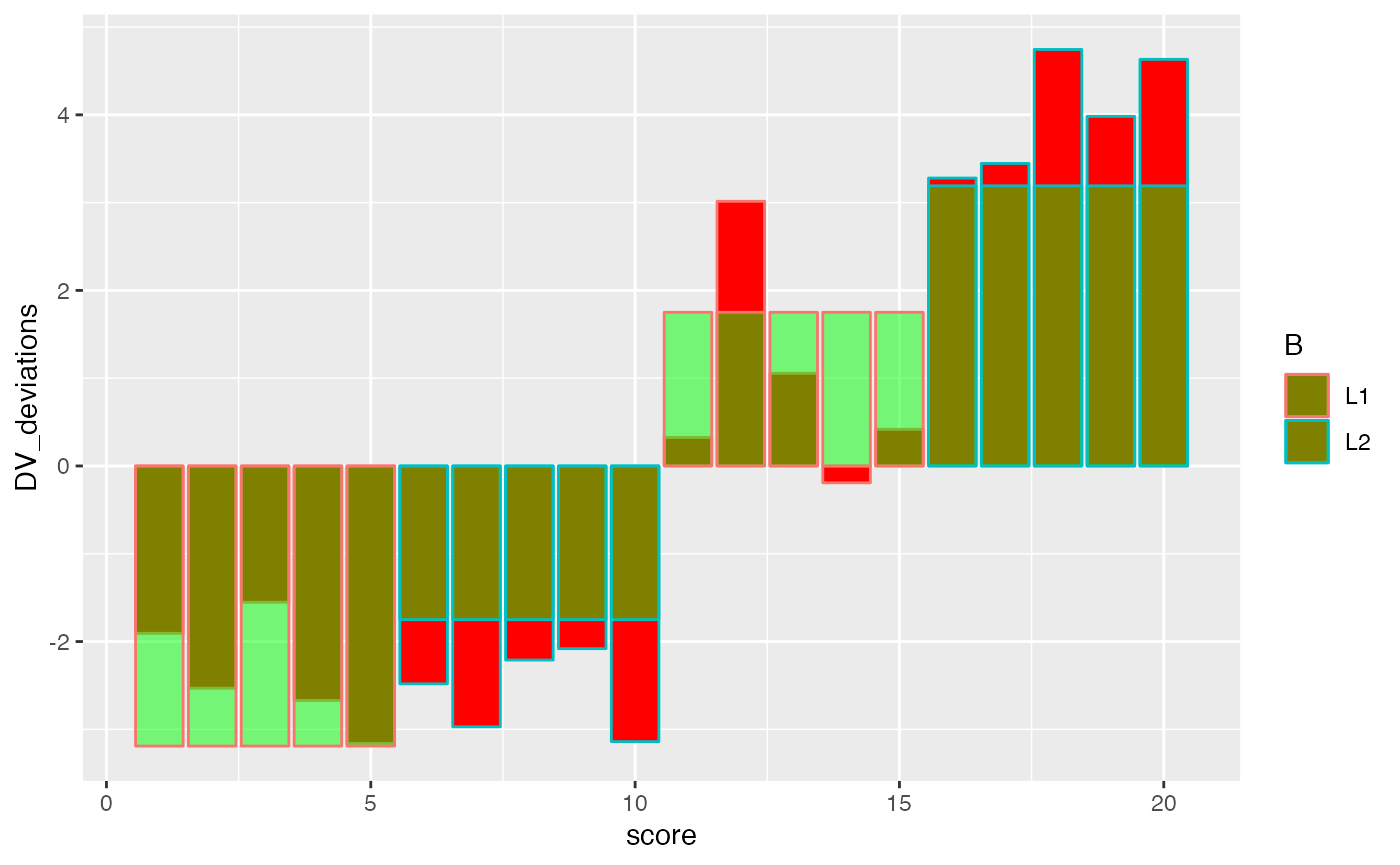
ggplot(factorial_data, aes(x=score, shape=A, color=B))+
  geom_bar(aes(y=DV_deviations), fill="red", stat="identity")+
  geom_bar(aes(y=A_deviations), fill="green", stat="identity", alpha=.5)
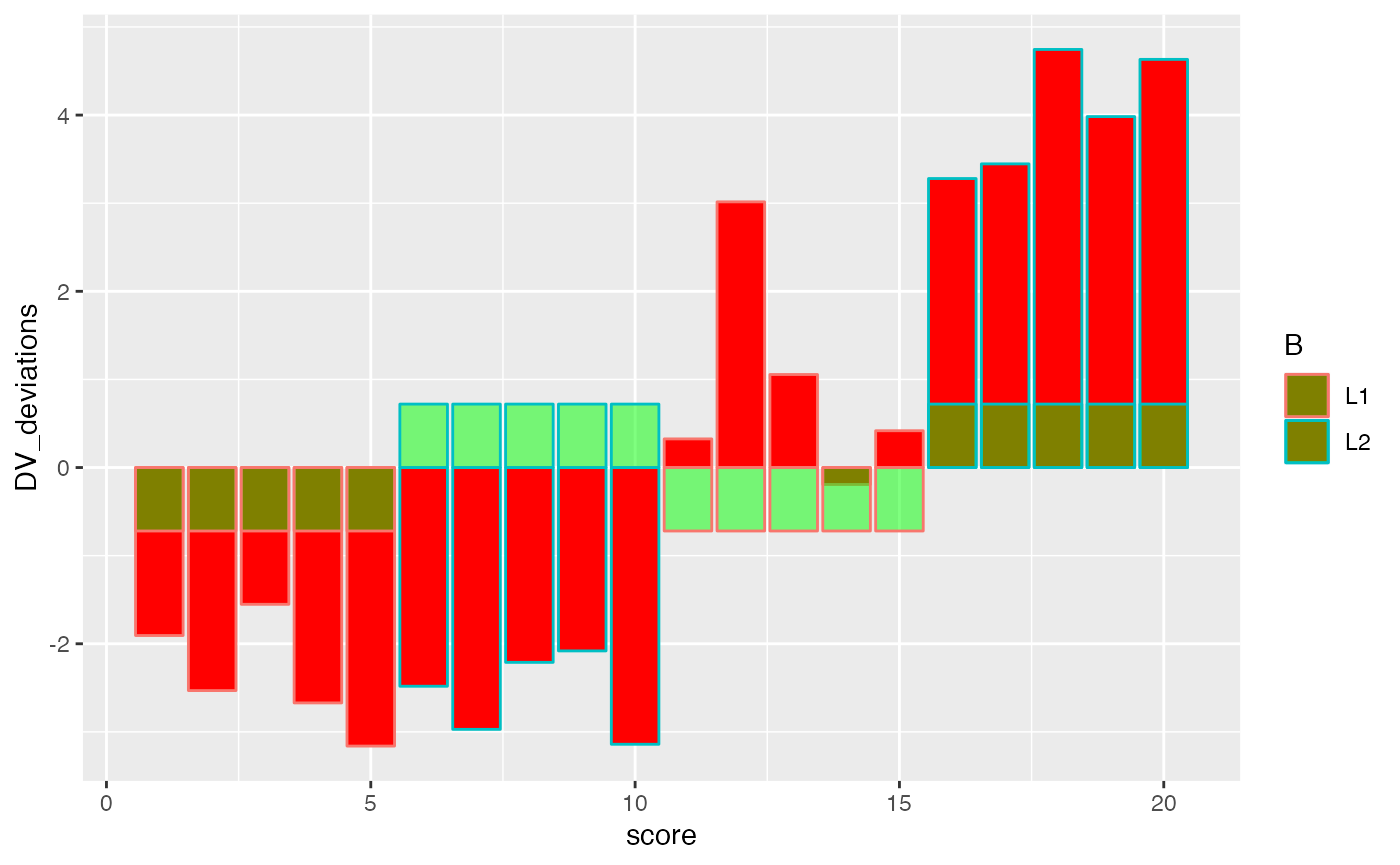
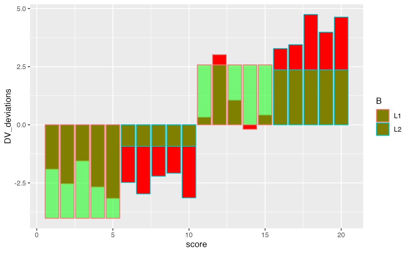
ggplot(factorial_data, aes(x=score, shape=A, color=B))+
  geom_bar(aes(y=DV_deviations), fill="red", stat="identity")+
  geom_bar(aes(y=B_deviations), fill="green", stat="identity", alpha=.5)
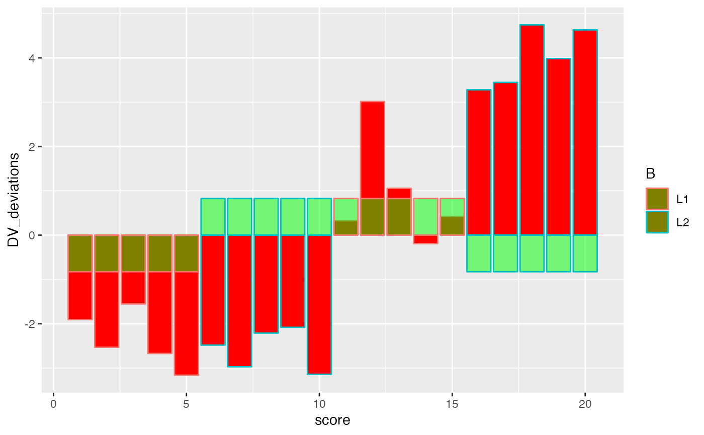
ggplot(factorial_data, aes(x=score, shape=A, color=B))+
  geom_bar(aes(y=DV_deviations), fill="red", stat="identity")+
  geom_bar(aes(y=cell_deviations), fill="green", stat="identity", alpha=.5)
ggplot(factorial_data, aes(x=score, shape=A, color=B))+
  geom_bar(aes(y=DV_deviations), fill="red", stat="identity")+
  geom_bar(aes(y=(A_deviations+B_deviations)), fill="green", stat="identity", alpha=.5)
ggplot(factorial_data, aes(x=score, shape=A, color=B))+
  geom_bar(aes(y=DV_deviations), fill="red", stat="identity")+
  geom_bar(aes(y=(A_deviations+B_deviations+cell_deviations)), fill="green", stat="identity", alpha=.5)
factorial_data <- factorial_data %>%
mutate(score = 1:(n*2))
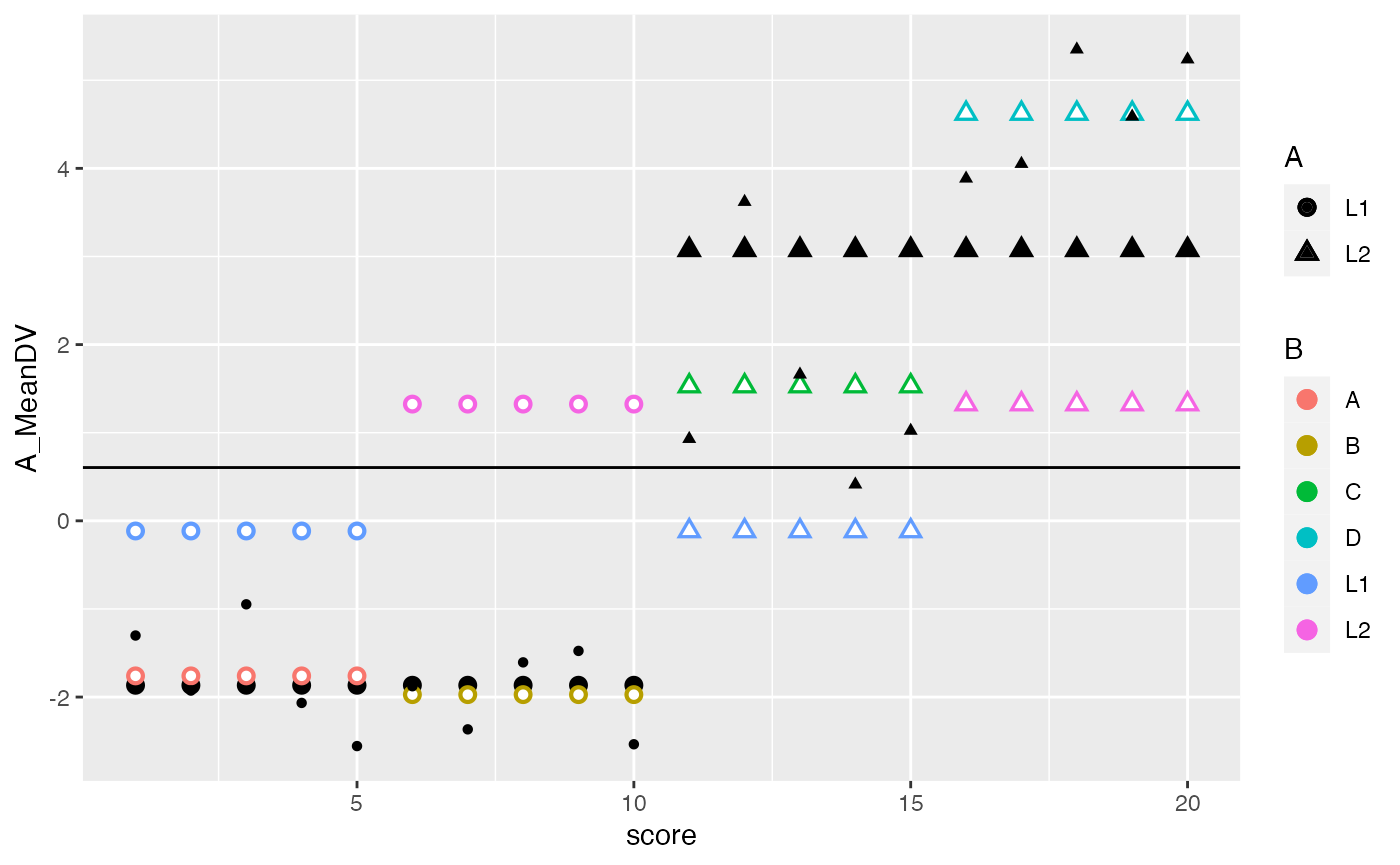
ggplot(factorial_data, aes(x=score, shape=A, color=B))+
geom_hline(yintercept = mean(factorial_data$DV))+
geom_point(aes(y=A_MeanDV), size= 3,color="black") +
geom_point(aes(y=B_MeanDV), size=3) +
geom_point(aes(y=B_MeanDV), color="white") +
geom_point(aes(y=cell_MeanDV,color=C), size=3) +
geom_point(aes(y=cell_MeanDV), color="white") +
geom_point(aes(y=DV), color="black")
## SS Total

ggplot(factorial_data, aes(x=score, shape=A, color=B))+
  geom_hline(yintercept = mean(factorial_data$DV))+
  geom_point(aes(y=A_MeanDV), size= 3,color="black") +
  geom_point(aes(y=B_MeanDV), size=3) +
  geom_point(aes(y=B_MeanDV), color="white") +
  geom_point(aes(y=cell_MeanDV,color=C), size=3) +
  geom_point(aes(y=cell_MeanDV), color="white") +
  geom_point(aes(y=DV), color="black") +
  geom_segment(aes(xend = score, y=grand_mean, yend = DV_deviations), alpha = .9, color="red")

## SS A
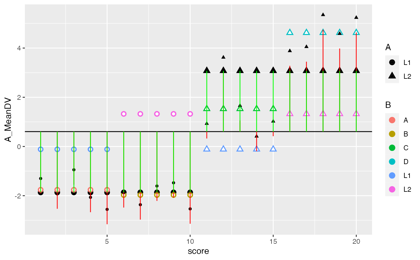
ggplot(factorial_data, aes(x=score, shape=A, color=B))+
geom_hline(yintercept = mean(factorial_data$DV))+
geom_point(aes(y=A_MeanDV), size= 3,color="black") +
geom_point(aes(y=B_MeanDV), size=3) +
geom_point(aes(y=B_MeanDV), color="white") +
geom_point(aes(y=cell_MeanDV,color=C), size=3) +
geom_point(aes(y=cell_MeanDV), color="white") +
geom_point(aes(y=DV), color="black") +
geom_segment(aes(xend = score, y=grand_mean, yend = DV_deviations), alpha = .9, color="red") +
geom_segment(aes(xend = score, y=grand_mean, yend = A_MeanDV), alpha = .9, color="green")
ggplot(factorial_data, aes(x=score, shape=A, color=B))+
  geom_hline(yintercept = mean(factorial_data$DV))+
  geom_point(aes(y=A_MeanDV), size= 3,color="black") +
  geom_point(aes(y=B_MeanDV), size=3) +
  geom_point(aes(y=B_MeanDV), color="white") +
  geom_point(aes(y=cell_MeanDV,color=C), size=3) +
  geom_point(aes(y=cell_MeanDV), color="white") +
  geom_point(aes(y=DV), color="black") +
  geom_segment(aes(xend = score, y=grand_mean, yend = DV_deviations), alpha = .9, color="red") +
  geom_segment(aes(xend = score, y=grand_mean, yend = B_MeanDV), alpha = .9, color="green")
ggplot(factorial_data, aes(x=score, shape=A, color=B))+
  geom_hline(yintercept = mean(factorial_data$DV))+
  geom_point(aes(y=A_MeanDV), size= 3,color="black") +
  geom_point(aes(y=B_MeanDV), size=3) +
  geom_point(aes(y=B_MeanDV), color="white") +
  geom_point(aes(y=cell_MeanDV,color=C), size=3) +
  geom_point(aes(y=cell_MeanDV), color="white") +
  geom_point(aes(y=DV), color="black") +
  geom_segment(aes(xend = score, y=grand_mean, yend = DV_deviations), alpha = .9, color="red") +
  geom_segment(aes(xend = score, y=grand_mean, yend = cell_MeanDV), alpha = .9, color="green")
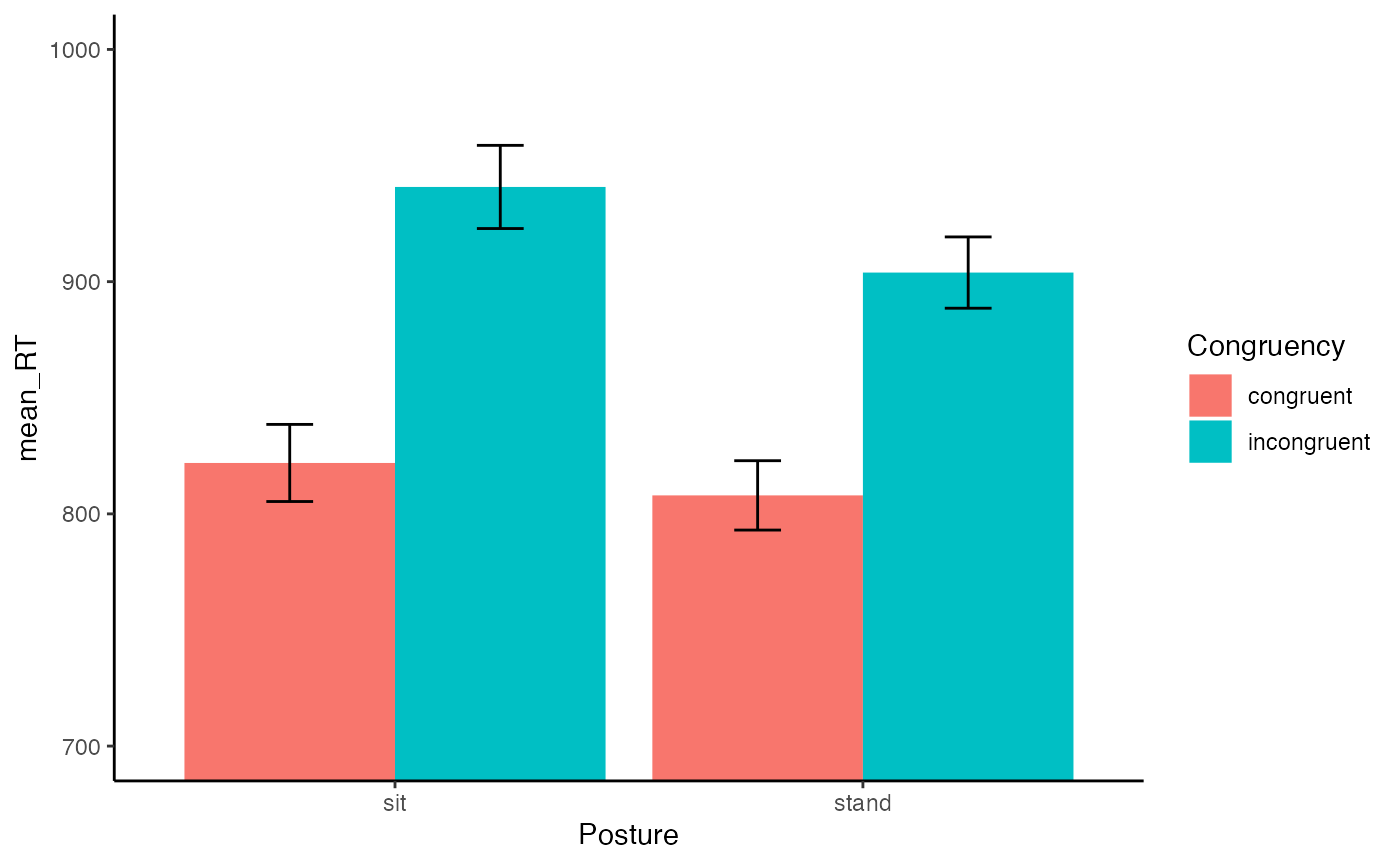
- Complete the 2x2 factorial lab found here https://crumplab.github.io/statisticsLab/lab-10-factorial-anova.html, up to section 10.4.8. More specifically, your task is to follow that lab exercise to load in the data, transform the data into long-format, conduct a 2x2 between subjects ANOVA, and write a short results section reporting the main effects and interaction. (3 points)
library(data.table)
#>
#> Attaching package: 'data.table'
#> The following objects are masked from 'package:dplyr':
#>
#> between, first, last
#> The following object is masked from 'package:purrr':
#>
#> transpose
all_data <- fread("data/stroop_stand.csv")
RTs <- c(as.numeric(unlist(all_data[,1])),
as.numeric(unlist(all_data[,2])),
as.numeric(unlist(all_data[,3])),
as.numeric(unlist(all_data[,4]))
)
Congruency <- rep(rep(c("Congruent","Incongruent"),each=50),2)
Posture <- rep(c("Stand","Sit"),each=100)
Subject <- rep(1:50,4)
stroop_df <- data.frame(Subject,Congruency,Posture,RTs)
library(tidyr)
stroop_long<- gather(all_data, key=Condition, value=RTs,
congruent_stand, incongruent_stand,
congruent_sit, incongruent_sit)
new_columns <- tstrsplit(stroop_long$Condition, "_", names=c("Congruency","Posture"))
stroop_long <- cbind(stroop_long,new_columns)
stroop_long <- cbind(stroop_long,Subject=rep(1:50,4))
library(dplyr)
library(ggplot2)
library(tidyr)
plot_means <- stroop_long %>%
group_by(Congruency,Posture) %>%
summarise(mean_RT = mean(RTs),
SEM = sd(RTs)/sqrt(length(RTs)))
#> �[1m�[22m`summarise()` has grouped output by 'Congruency'. You can override using the
#> `.groups` argument.
ggplot(plot_means, aes(x=Posture, y=mean_RT, group=Congruency, fill=Congruency))+
geom_bar(stat="identity", position="dodge")+
geom_errorbar(aes(ymin=mean_RT-SEM, ymax=mean_RT+SEM),
position=position_dodge(width=0.9),
width=.2)+
theme_classic()+
coord_cartesian(ylim=c(700,1000))
aov_out<-aov(RTs ~ Congruency*Posture, stroop_long)
summary_out<-summary(aov_out)
summary_out
#>                     Df  Sum Sq Mean Sq F value   Pr(>F)
#> Congruency           1  576822  576822  43.734 3.49e-10 ***
#> Posture              1   32303   32303   2.449    0.119
#> Congruency:Posture   1    6560    6560   0.497    0.481
#> Residuals          196 2585080   13189
#> ---
#> Signif. codes:  0 '***' 0.001 '**' 0.01 '*' 0.05 '.' 0.1 ' ' 1
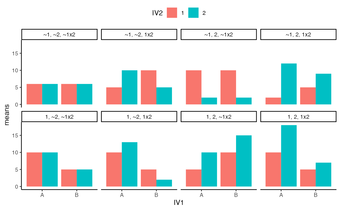
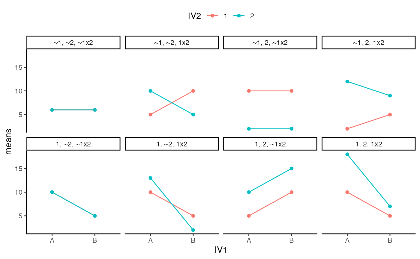
- In chapter 10 of Crump et al. (2018), there is a discussion of patterns of main effects and interactions that can occur in a 2x2 design, which represents perhaps the simplest factorial design. There are 8 possible outcomes discussed https://crumplab.github.io/statistics/more-on-factorial-designs.html#looking-at-main-effects-and-interactions. Examples of these 8 outcomes are shown in two figures, one with bar graphs, and one with line graphs. Reproduce either of these figures using ggplot2. (3 points)
p1<- data.frame(IV1 = c("A","A","B","B"),
                IV2 = c("1","2","1","2"),
                means = c(6,6,6,6))
p2<- data.frame(IV1 = c("A","A","B","B"),
                IV2 = c("1","2","1","2"),
                means = c(10,10,5,5))
p3<- data.frame(IV1 = c("A","A","B","B"),
                IV2 = c("1","2","1","2"),
                means = c(10,13,5,2))
p4<- data.frame(IV1 = c("A","A","B","B"),
                IV2 = c("1","2","1","2"),
                means = c(5,10,10,15))
p5<- data.frame(IV1 = c("A","A","B","B"),
                IV2 = c("1","2","1","2"),
                means = c(10,18,5,7))
p6<- data.frame(IV1 = c("A","A","B","B"),
                IV2 = c("1","2","1","2"),
                means = c(10,2,10,2))
p7<- data.frame(IV1 = c("A","A","B","B"),
                IV2 = c("1","2","1","2"),
                means = c(2,12,5,9))
p8<- data.frame(IV1 = c("A","A","B","B"),
                IV2 = c("1","2","1","2"),
                means = c(5,10,10,5))
all_22s <- rbind(p1,p2,p3,p4,p5,p6,p7,p8)
type <- c(rep("~1, ~2, ~1x2",4),
          rep("1, ~2, ~1x2",4),
          rep("1, ~2, 1x2",4),
          rep("1, 2, ~1x2",4),
          rep("1, 2, 1x2",4),
          rep("~1, 2, ~1x2",4),
          rep("~1, 2, 1x2",4),
          rep("~1, ~2, 1x2",4))
type<-as.factor(type)
all_22s <- cbind(all_22s,type)
ggplot(all_22s, aes(x=IV1, y=means, group=IV2, fill=IV2))+
  geom_bar(stat="identity", position="dodge")+
  theme_classic()+
  facet_wrap(~type, nrow=2)+
  theme(legend.position = "top")
ggplot(all_22s, aes(x=IV1, y=means, group=IV2, color=IV2))+
  geom_point()+
  geom_line()+
  theme_classic()+
  facet_wrap(~type, nrow=2)+
  theme(legend.position = "top")
- In the conceptual section of this lab we used an R simulation to find the family-wise type I error rate for a simple factorial design with 2 independent variables. Use an R simulation to find the family-wise type I error rate for a factorial design with 3 independent variables. (3 points)
sims <- rbinom(10000,7,.05)
length(sims[sims > 0])/10000
#> [1] 0.2907

save_sim <- tibble()

# loop to conduct i number of simulations
for(i in 1:10000){

  #simulate null data for a 2x2
  n <- 12
  factorial_data <- tibble(A = factor(rep(c("L1","L2"), each = n)),
                         B = factor(rep(rep(c("L1","L2"), each = n/2),2)),
                         C = factor(rep(c("L1","L2"), n)),
                         DV = rnorm(n*2,0,1))
  # compute ANOVA
  output <- summary(aov(DV ~ A*B*C, data = factorial_data))

  #save p-values for each effect
  sim_tibble <- tibble(p_vals = output[[1]]$`Pr(>F)`[1:7],
                       effect = c("A","B","C","AxB","AxC","BxC","AxBxC"),
                       sim = rep(i,7))

  #add the saved values to the overall tibble
  save_sim <-rbind(save_sim,sim_tibble)
}

type_I_errors <- save_sim %>%
  filter(p_vals < .05) %>%
  group_by(sim) %>%
  count()

dim(type_I_errors)[1]/10000
#> [1] 0.2767
- Show that a 2x2 factorial ANOVA can be accomplished by using a one-factor ANOVA with three linear contrasts. (3 points)
library(tibble)
library(dplyr)

n <- 10
factorial_data <- tibble(A = factor(rep(c("L1","L2"), each = n)),
                         B = factor(rep(rep(c("L1","L2"), each = n/2),2)),
                         DV = rnorm(n*2,0,1))

aov_out <- aov(DV ~ A*B, data = factorial_data)
summary(aov_out)
#>             Df Sum Sq Mean Sq F value Pr(>F)
#> A            1  0.008  0.0079   0.010 0.9227
#> B            1  0.903  0.9026   1.105 0.3088
#> A:B          1  2.954  2.9539   3.616 0.0754 .
#> Residuals   16 13.071  0.8170
#> ---
#> Signif. codes:  0 '***' 0.001 '**' 0.01 '*' 0.05 '.' 0.1 ' ' 1

factorial_data <- factorial_data %>%
  mutate(C = factor(rep(c("A","B","C","D"), each = n/2)))

# define your new set of contrasts

c1 <- c(1,1,-1,-1)
c2 <- c(1,-1,1,-1)
c3 <- c(1,-1,-1,1)


# combine them into the columns of a matrix
my_contrasts <- cbind(c1, c2, c3)

# assign them to the contrast property for your IV
contrasts(factorial_data$C) <- my_contrasts

aov_out <- aov(DV ~ C, data = factorial_data)

(full_summary <- summary.aov(aov_out,
                             split=list(C=list("A"=1,
                                                "B" = 2,
                                                "A:B"= 3)
                                        )
                             )
  )
#>             Df Sum Sq Mean Sq F value Pr(>F)
#> C            3  3.864  1.2881   1.577 0.2340
#>   C: A       1  0.008  0.0079   0.010 0.9227
#>   C: B       1  0.903  0.9026   1.105 0.3088
#>   C: A:B     1  2.954  2.9539   3.616 0.0754 .
#> Residuals   16 13.071  0.8170
#> ---
#> Signif. codes:  0 '***' 0.001 '**' 0.01 '*' 0.05 '.' 0.1 ' ' 1