Lab8

Consider a 2x2 design. Assume the DV is measured from a normal distribution with mean 0, and standard deviation 1. Assume that the main effect of A causes a total shift of .5 standard deviations of the mean between the levels. Assume that level 1 of B is a control, where you expect to measure the standard effect of A. Assume that level 2 of B is an experimental factor intended to reduce the effect of A by .25 standard deviations.

A. create a ggplot2 figure that depicts the expected results from this design (2 points)

library(tidyverse)
#> ── Attaching packages ─────────────────────────────────────── tidyverse 1.3.1 ──
#> ✓ ggplot2 3.3.5     ✓ purrr   0.3.4
#> ✓ tibble  3.1.6     ✓ dplyr   1.0.7
#> ✓ tidyr   1.2.0     ✓ stringr 1.4.0
#> ✓ readr   2.0.2     ✓ forcats 0.5.1
#> Warning: package 'tidyr' was built under R version 4.1.2
#> ── Conflicts ────────────────────────────────────────── tidyverse_conflicts() ──
#> x dplyr::filter() masks stats::filter()
#> x dplyr::lag()    masks stats::lag()

df <- data.frame(A = c("A1","A1","A2","A2"),
                 B = c(1,2,1,2),
                 dv = c(0,0,0.5,0.25)
)

ggplot(df, aes(y=dv, x=B, fill = A)) +
  geom_bar(stat = "identity", position = "dodge")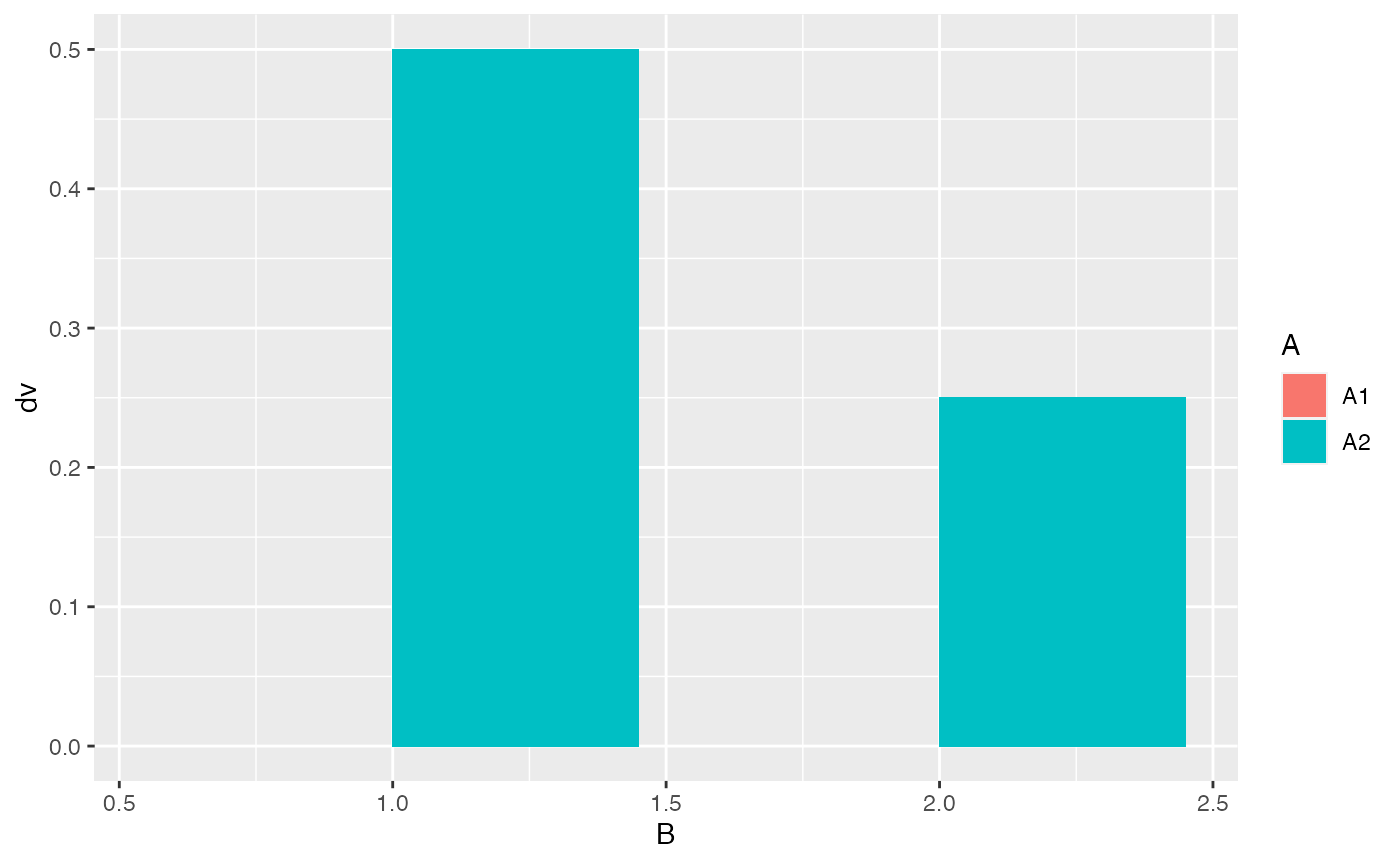

ggplot(df, aes(y=dv, x=B, color = A)) +
  geom_point()+
  geom_line()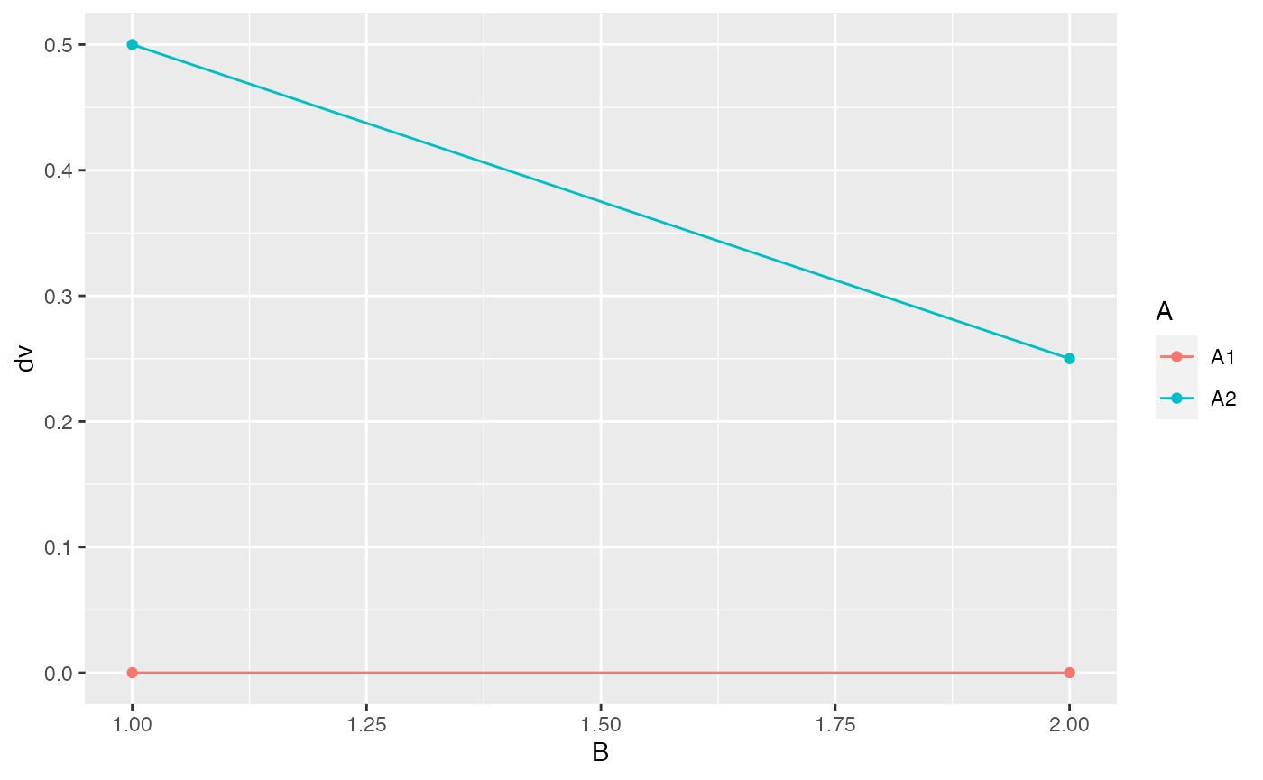

Conduct simulation-based power analyses to answer the questions.

B. How many subjects are needed to detect the main effect of A with power = .8? (2 points)

# N per group
N <- 60

A_pvalue <- c()
B_pvalue <- c()
AB_pvalue <- c()
for(i in 1:1000){
  IVA <- rep(rep(c("1","2"), each=2),N)
  IVB <- rep(rep(c("1","2"), 2),N)
  DV <- c(replicate(N,c(rnorm(1,0,1), # means A1B1
                        rnorm(1,0,1), # means A1B2
                        rnorm(1,.5,1), # means A2B1
                        rnorm(1,.25,1)  # means A2B2
          )))
  sim_df <- data.frame(IVA,IVB,DV)
  
  aov_results <- summary(aov(DV~IVA*IVB, sim_df))
  A_pvalue[i]<-aov_results[[1]]$`Pr(>F)`[1]
  B_pvalue[i]<-aov_results[[1]]$`Pr(>F)`[2]
  AB_pvalue[i]<-aov_results[[1]]$`Pr(>F)`[3]
}

length(A_pvalue[A_pvalue<0.05])/1000
#> [1] 0.802
length(B_pvalue[B_pvalue<0.05])/1000
#> [1] 0.164
length(AB_pvalue[AB_pvalue<0.05])/1000
#> [1] 0.16

C. How many subjects are needed to detect the interaction effect with power = .8? (2 points)

# N per group
N <- 525

A_pvalue <- c()
B_pvalue <- c()
AB_pvalue <- c()
for(i in 1:1000){
  IVA <- rep(rep(c("1","2"), each=2),N)
  IVB <- rep(rep(c("1","2"), 2),N)
  DV <- c(replicate(N,c(rnorm(1,0,1), # means A1B1
                        rnorm(1,0,1), # means A1B2
                        rnorm(1,.5,1), # means A2B1
                        rnorm(1,.25,1)  # means A2B2
          )))
  sim_df <- data.frame(IVA,IVB,DV)
  
  aov_results <- summary(aov(DV~IVA*IVB, sim_df))
  A_pvalue[i]<-aov_results[[1]]$`Pr(>F)`[1]
  B_pvalue[i]<-aov_results[[1]]$`Pr(>F)`[2]
  AB_pvalue[i]<-aov_results[[1]]$`Pr(>F)`[3]
}

length(A_pvalue[A_pvalue<0.05])/1000
#> [1] 1
length(B_pvalue[B_pvalue<0.05])/1000
#> [1] 0.817
length(AB_pvalue[AB_pvalue<0.05])/1000
#> [1] 0.813

Bonus point question:

Create a power curve showing how power for the interaction effect in this example is influenced by number of subjects. Choose a range of N from 25 to 800 (per cell) and run a simulation-based power analysis for increments of 25 subjects. Then plot the results using ggplot2 (2 points).