Analysis E3 Delayed Auditory Feedback

Matt

5/14/2019

Load Libraries

library(papaja)
library(TalkTyping)
library(dplyr)
library(Crump)
library(xtable)
library(ggplot2)
library(ggpubr)
library(forcats)

E3 IKSI Analysis

#load E2 data
E3_data <- talk_type_E3_data

# IKSI analysis

E3_data <- E3_data %>%
           filter(letter_accuracy == 1,
                           iksis < 5000,
                           LetterType != "Space") %>%
            mutate(subject = as.factor(subject),
                   suppression = as.factor(delay),
                   LetterType = as.factor(LetterType)) %>%
            group_by(subject,delay,LetterType) %>%
            summarise(mean_iksi = mean(modified_recursive_moving(iksis)$restricted),
                      prop_removed = modified_recursive_moving(iksis)$prop_removed)
                  
E3_aov_out <- aov(mean_iksi ~ delay*LetterType + 
                    Error(subject/(delay*LetterType)), E3_data)

knitr::kable(xtable(summary(E3_aov_out)))

	Df	Sum Sq	Mean Sq	F value	Pr(>F)
Residuals	17	3853286.03	226663.884	NA	NA
delay	5	10034.50	2006.899	1.561962	0.1796028
Residuals1	85	109212.88	1284.857	NA	NA
LetterType	1	3754354.76	3754354.761	30.123375	0.0000400
Residuals	17	2118754.29	124632.605	NA	NA
delay:LetterType	5	11740.34	2348.068	1.834162	0.1147653
Residuals	85	108815.78	1280.186	NA	NA

E3_apa_print <- apa_print(E3_aov_out)
E3_means <- model.tables(E3_aov_out,"means")

First Letter one-way with linear contrasts

#load E3 data
E3_data <- talk_type_E3_data

# IKSI analysis

#E3_data$suppression <- fct_relevel(E3_data$suppression,c("Normal","SayThe","TueThur","Alphabet","RandLetter","Count"))

E3_data <- E3_data %>%
           filter(letter_accuracy == 1,
                           iksis < 5000,
                           LetterType != "Space") %>%
            mutate(subject = as.factor(subject),
                   delay = as.factor(delay),
                   LetterType = as.factor(LetterType)) %>%
            group_by(subject,delay,LetterType) %>%
            summarise(mean_iksi = mean(modified_recursive_moving(iksis)$restricted),
                      prop_removed = modified_recursive_moving(iksis)$prop_removed)

E3_FL_data <- E3_data %>%
                filter(LetterType == "First")

E3_FL_aov_out <- aov(mean_iksi ~ delay + 
                    Error(subject/(delay)), E3_FL_data)

knitr::kable(xtable(summary(E3_FL_aov_out)))

	Df	Sum Sq	Mean Sq	F value	Pr(>F)
Residuals	17	5789564.77	340562.634	NA	NA
delay	5	21375.17	4275.033	1.708016	0.1415004
Residuals1	85	212748.49	2502.923	NA	NA

E3_FL_apa_print <- apa_print(E3_FL_aov_out)
E3_FL_means <- model.tables(E3_FL_aov_out,"means")

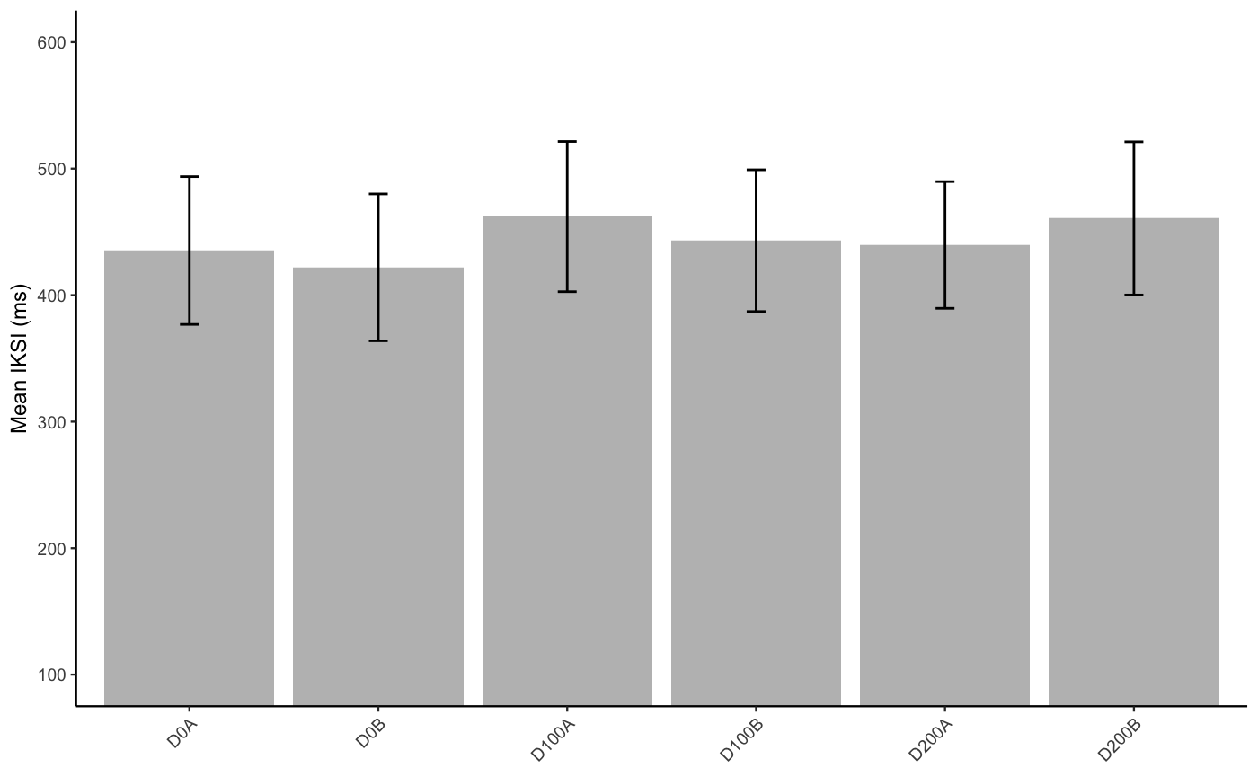
Plot

E3_FL_iksi_table <- E3_FL_data %>%
              group_by(delay) %>%
              summarize(mIKSI = mean(mean_iksi),
                        sem = sd(mean_iksi)/sqrt(length(mean_iksi)))

E3_FL_graph_iksi <- ggplot(E3_FL_iksi_table, aes(x=delay,
                                             y=mIKSI))+
  geom_bar(stat="identity", position="dodge", fill="grey")+
  geom_errorbar(aes(ymin=mIKSI-sem,
                    ymax=mIKSI+sem), width=.1,
                linetype="solid", position=position_dodge(.9))+
  scale_fill_grey(start = 0.6, end = 0.8, na.value = "red",
  aesthetics = "fill")+
  theme_classic(base_size=9)+
  theme(legend.position = "top",
        legend.title = element_blank())+
  coord_cartesian(ylim=c(100,600))+
  scale_y_continuous(minor_breaks=seq(100,600,25),
                     breaks=seq(100,600,100))+
   #scale_x_discrete(labels = c('Normal',
  #                            'Letter',
  #                            'Word',
  #                            'Letter',
  #                            'Word'))+
  ylab("Mean IKSI (ms)")+
  theme(axis.title.x = element_blank())+
  theme(axis.text.x = element_text(angle = 45, hjust = 1))
 # facet_wrap(~delay, scales = "free_x",
 #            strip.position="bottom")

knitr::kable(E3_FL_iksi_table)

delay	mIKSI	sem
D0A	435.2722	58.41954
D0B	421.9304	58.03721
D100A	462.0889	59.35957
D100B	443.0553	56.01902
D200A	439.6609	50.08614
D200B	460.6623	60.53042

E3_FL_graph_iksi

Middle Letter one-way with linear contrasts

#load E3 data
E3_data <- talk_type_E3_data

# IKSI analysis

#E3_data$delay <- fct_relevel(E3_data$delay,c("Normal","SayThe","TueThur","Alphabet","RandLetter","Count"))

E3_data <- E3_data %>%
           filter(letter_accuracy == 1,
                           iksis < 5000,
                           LetterType != "Space") %>%
            mutate(subject = as.factor(subject),
                   delay = as.factor(delay),
                   LetterType = as.factor(LetterType)) %>%
            group_by(subject,delay,LetterType) %>%
            summarise(mean_iksi = mean(modified_recursive_moving(iksis)$restricted),
                      prop_removed = modified_recursive_moving(iksis)$prop_removed)

E3_ML_data <- E3_data %>%
                filter(LetterType == "Middle")

E3_ML_aov_out <- aov(mean_iksi ~ delay + 
                    Error(subject/(delay)), E3_ML_data)

knitr::kable(xtable(summary(E3_ML_aov_out)))

	Df	Sum Sq	Mean Sq	F value	Pr(>F)
Residuals	17	182475.5535	10733.85609	NA	NA
delay	5	399.6713	79.93426	1.286779	0.2772062
Residuals1	85	5280.1711	62.11966	NA	NA

E3_ML_apa_print <- apa_print(E3_ML_aov_out)
E3_ML_means <- model.tables(E3_ML_aov_out,"means")

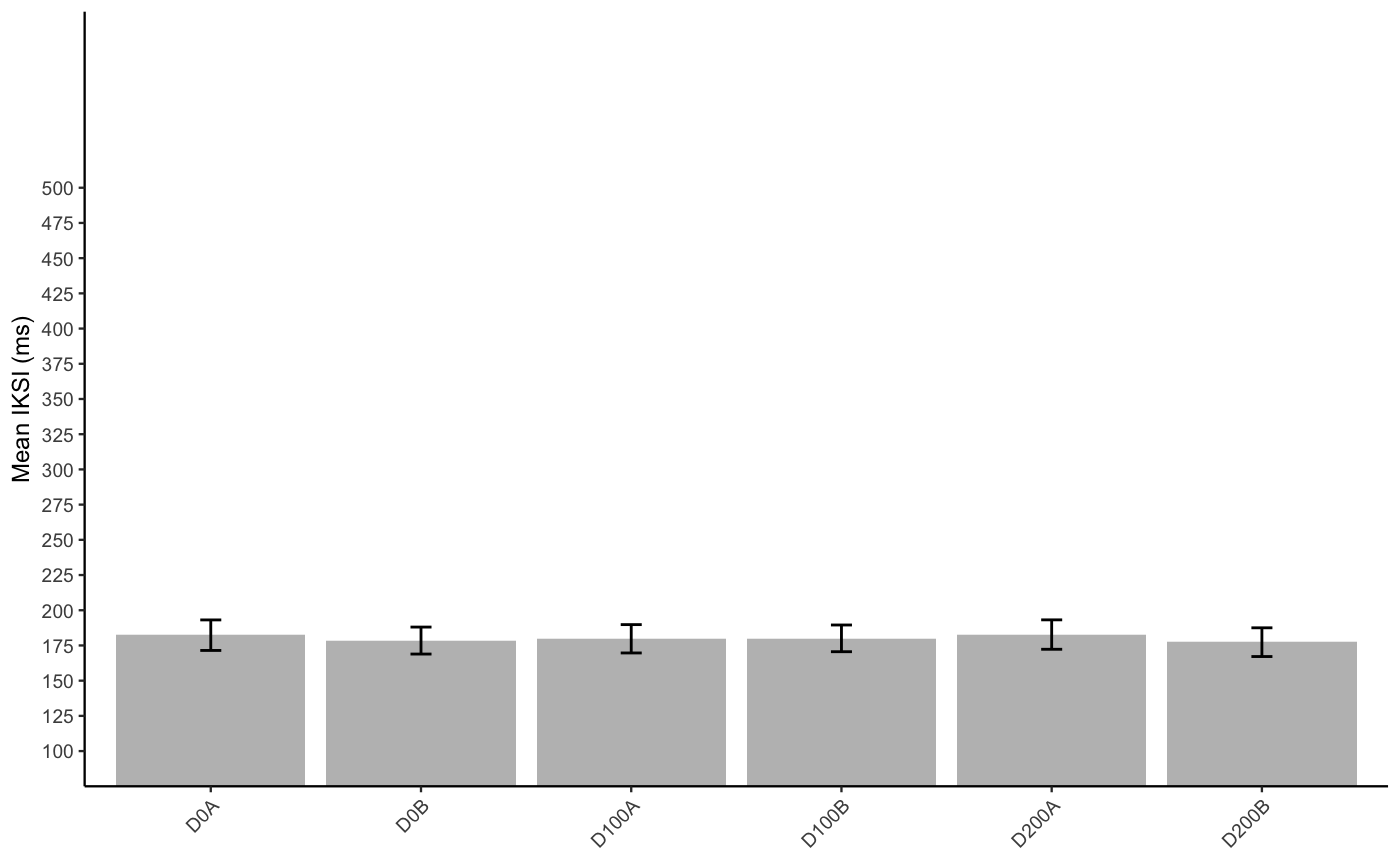
Plot

E3_ML_iksi_table <- E3_ML_data %>%
              group_by(delay) %>%
              summarize(mIKSI = mean(mean_iksi),
                        sem = sd(mean_iksi)/sqrt(length(mean_iksi)))

E3_ML_graph_iksi <- ggplot(E3_ML_iksi_table, aes(x=delay,
                                             y=mIKSI))+
  geom_bar(stat="identity", position="dodge", fill="grey")+
  geom_errorbar(aes(ymin=mIKSI-sem,
                    ymax=mIKSI+sem), width=.1,
                linetype="solid", position=position_dodge(.9))+
  scale_fill_grey(start = 0.6, end = 0.8, na.value = "red",
  aesthetics = "fill")+
  theme_classic(base_size=9)+
  theme(legend.position = "top",
        legend.title = element_blank())+
  coord_cartesian(ylim=c(100,600))+
  scale_y_continuous(minor_breaks=seq(100,600,100),
                     breaks=seq(100,500,25))+
   #scale_x_discrete(labels = c('Normal',
  #                            'Letter',
  #                            'Word',
  #                            'Letter',
  #                            'Word'))+
  ylab("Mean IKSI (ms)")+
  theme(axis.title.x = element_blank())+
  theme(axis.text.x = element_text(angle = 45, hjust = 1))
 # facet_wrap(~delay, scales = "free_x",
 #            strip.position="bottom")

knitr::kable(E3_ML_iksi_table)

delay	mIKSI	sem
D0A	182.2944	10.836945
D0B	178.4739	9.581092
D100A	179.7358	10.064446
D100B	180.0463	9.481460
D200A	182.7333	10.446362
D200B	177.3297	10.199338

E3_ML_graph_iksi

First Letter Accuracy one-way with linear contrasts

#load E3 data
E3_data <- talk_type_E3_data

# IKSI analysis

#E3_data$delay <- fct_relevel(E3_data$delay,c("Normal","SayThe","TueThur","Alphabet","RandLetter","Count"))

E3_data <- E3_data %>%
           filter(LetterType != "Space") %>%
            mutate(subject = as.factor(subject),
                   delay = as.factor(delay),
                   LetterType = as.factor(LetterType)) %>%
            group_by(subject,delay,LetterType) %>%
            summarise(mean_acc = mean(letter_accuracy))

E3acc_FL_data <- E3_data %>%
                filter(LetterType == "First")

E3acc_FL_aov_out <- aov(mean_acc ~ delay + 
                    Error(subject/(delay)), E3acc_FL_data)

knitr::kable(xtable(summary(E3acc_FL_aov_out)))

	Df	Sum Sq	Mean Sq	F value	Pr(>F)
Residuals	17	0.1216577	0.0071563	NA	NA
delay	5	0.0084619	0.0016924	2.71554	0.0251803
Residuals1	85	0.0529738	0.0006232	NA	NA

E3acc_FL_apa_print <- apa_print(E3acc_FL_aov_out)
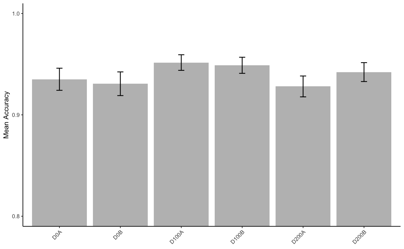
E3acc_FL_means <- model.tables(E3acc_FL_aov_out,"means")

Plot

E3acc_FL_table <- E3acc_FL_data %>%
              group_by(delay) %>%
              summarize(mAcc = mean(mean_acc),
                        sem = sd(mean_acc)/sqrt(length(mean_acc)))

E3acc_FL_graph_acc <- ggplot(E3acc_FL_table, aes(x=delay,
                                             y=mAcc))+
  geom_bar(stat="identity", position="dodge", fill="grey")+
  geom_errorbar(aes(ymin=mAcc-sem,
                    ymax=mAcc+sem), width=.1,
                linetype="solid", position=position_dodge(.9))+
  scale_fill_grey(start = 0.6, end = 0.8, na.value = "red",
  aesthetics = "fill")+
  theme_classic(base_size=9)+
  theme(legend.position = "top",
        legend.title = element_blank())+
  coord_cartesian(ylim=c(0.8,1))+
  scale_y_continuous(minor_breaks=seq(0.8,1,.1),
                     breaks=seq(0.8,1,.1))+
   #scale_x_discrete(labels = c('Normal',
  #                            'Letter',
  #                            'Word',
  #                            'Letter',
  #                            'Word'))+
  ylab("Mean Accuracy")+
  theme(axis.title.x = element_blank())+
  theme(axis.text.x = element_text(angle = 45, hjust = 1))
 # facet_wrap(~delay, scales = "free_x",
 #            strip.position="bottom")

knitr::kable(E3acc_FL_table)

delay	mAcc	sem
D0A	0.9351140	0.0109046
D0B	0.9306945	0.0116846
D100A	0.9516116	0.0076979
D100B	0.9488970	0.0079384
D200A	0.9280502	0.0102950
D200B	0.9421968	0.0093267

E3acc_FL_graph_acc

contrasts

# 0 vs 100

E3acc_FL_0vs100 <- apa_print(t_contrast_rm(df=E3acc_FL_data,
                             subject = "subject",
                             dv = "mean_acc",
                             condition = "delay",
                             A_levels = c("D0A","D0B"),
                             B_levels = c("D100A","D100B"),
                             contrast_weights = c(-1/2,-1/2,1/2,1/2) ))

## 
##  One Sample t-test
## 
## data:  contrast_vector
## t = 2.3379, df = 17, p-value = 0.03187
## alternative hypothesis: true mean is not equal to 0
## 95 percent confidence interval:
##  0.001692732 0.033007330
## sample estimates:
##  mean of x 
## 0.01735003

# 0 vs 200

E3acc_FL_0vs200 <- apa_print(t_contrast_rm(df=E3acc_FL_data,
                             subject = "subject",
                             dv = "mean_acc",
                             condition = "delay",
                             A_levels = c("D0A","D0B"),
                             B_levels = c("D200A","D200B"),
                             contrast_weights = c(-1/2,-1/2,1/2,1/2) ))

## 
##  One Sample t-test
## 
## data:  contrast_vector
## t = 0.39514, df = 17, p-value = 0.6977
## alternative hypothesis: true mean is not equal to 0
## 95 percent confidence interval:
##  -0.009630216  0.014068772
## sample estimates:
##   mean of x 
## 0.002219278

# 200 vs 100

E3acc_FL_200vs100 <- apa_print(t_contrast_rm(df=E3acc_FL_data,
                             subject = "subject",
                             dv = "mean_acc",
                             condition = "delay",
                             A_levels = c("D200A","D200B"),
                             B_levels = c("D100A","D100B"),
                             contrast_weights = c(-1/2,-1/2,1/2,1/2) ))

## 
##  One Sample t-test
## 
## data:  contrast_vector
## t = 2.3633, df = 17, p-value = 0.03029
## alternative hypothesis: true mean is not equal to 0
## 95 percent confidence interval:
##  0.001622903 0.028638602
## sample estimates:
##  mean of x 
## 0.01513075

Middle Letter Accuracy one-way with linear contrasts

#load E3 data
E3_data <- talk_type_E3_data

# IKSI analysis

#E3_data$delay <- fct_relevel(E3_data$delay,c("Normal","SayThe","TueThur","Alphabet","RandLetter","Count"))

E3_data <- E3_data %>%
           filter(LetterType != "Space") %>%
            mutate(subject = as.factor(subject),
                   delay = as.factor(delay),
                   LetterType = as.factor(LetterType)) %>%
            group_by(subject,delay,LetterType) %>%
            summarise(mean_acc = mean(letter_accuracy))

E3acc_ML_data <- E3_data %>%
                filter(LetterType == "Middle")

E3acc_ML_aov_out <- aov(mean_acc ~ delay + 
                    Error(subject/(delay)), E3acc_ML_data)

knitr::kable(xtable(summary(E3acc_ML_aov_out)))

	Df	Sum Sq	Mean Sq	F value	Pr(>F)
Residuals	17	0.4523198	0.0266070	NA	NA
delay	5	0.0203193	0.0040639	2.666947	0.027417
Residuals1	85	0.1295221	0.0015238	NA	NA

E3acc_ML_apa_print <- apa_print(E3acc_ML_aov_out)
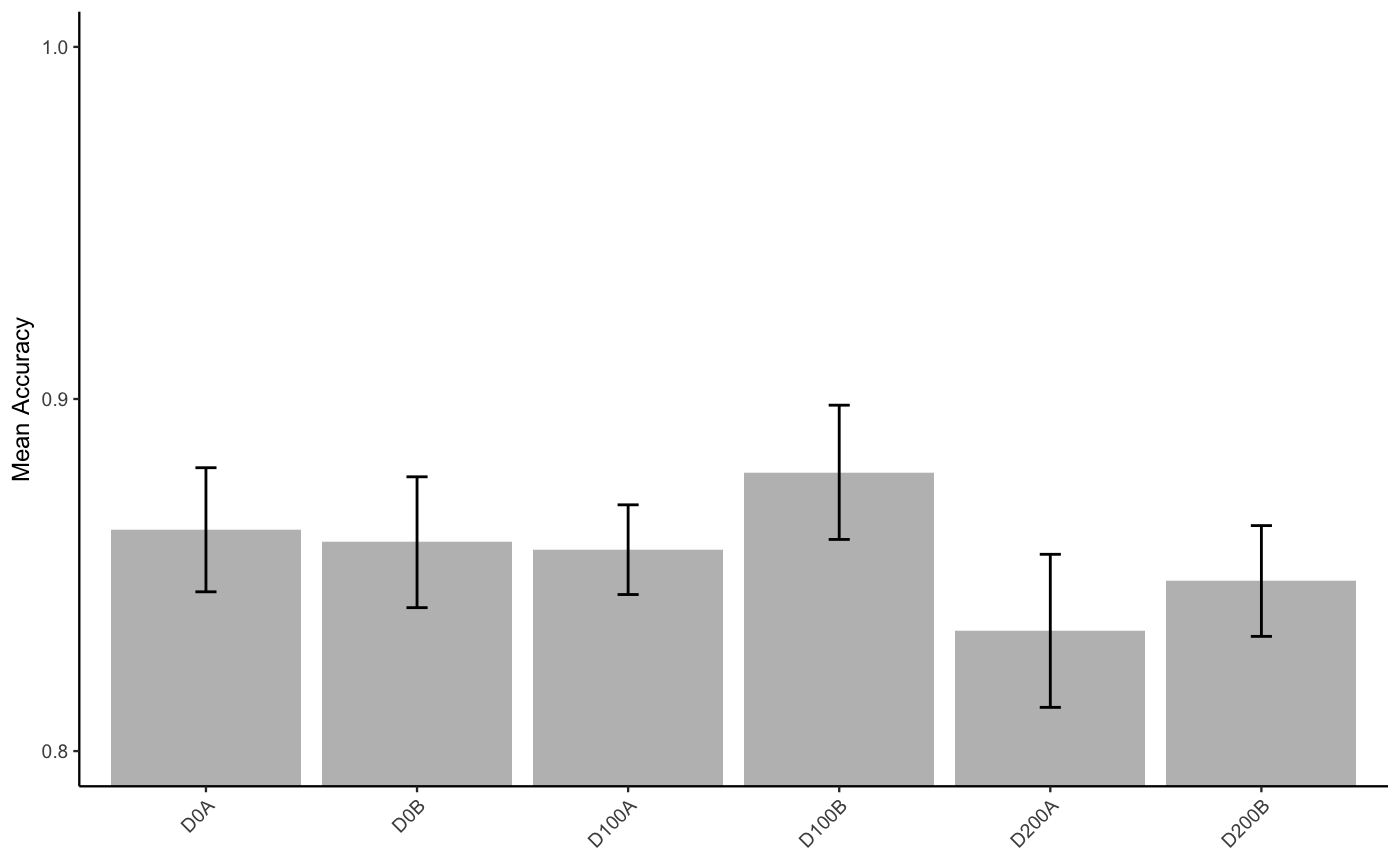
E3acc_ML_means <- model.tables(E3acc_ML_aov_out,"means")

Plot

E3acc_ML_table <- E3acc_ML_data %>%
              group_by(delay) %>%
              summarize(mAcc = mean(mean_acc),
                        sem = sd(mean_acc)/sqrt(length(mean_acc)))

E3acc_ML_graph_acc <- ggplot(E3acc_ML_table, aes(x=delay,
                                             y=mAcc))+
  geom_bar(stat="identity", position="dodge", fill="grey")+
  geom_errorbar(aes(ymin=mAcc-sem,
                    ymax=mAcc+sem), width=.1,
                linetype="solid", position=position_dodge(.9))+
  scale_fill_grey(start = 0.6, end = 0.8, na.value = "red",
  aesthetics = "fill")+
  theme_classic(base_size=9)+
  theme(legend.position = "top",
        legend.title = element_blank())+
  coord_cartesian(ylim=c(0.8,1))+
  scale_y_continuous(minor_breaks=seq(0.8,1,.1),
                     breaks=seq(0.8,1,.1))+
   #scale_x_discrete(labels = c('Normal',
  #                            'Letter',
  #                            'Word',
  #                            'Letter',
  #                            'Word'))+
  ylab("Mean Accuracy")+
  theme(axis.title.x = element_blank()) +
  theme(axis.text.x = element_text(angle = 45, hjust = 1))
 # facet_wrap(~delay, scales = "free_x",
 #            strip.position="bottom")

knitr::kable(E3acc_ML_table)

delay	mAcc	sem
D0A	0.8628590	0.0176220
D0B	0.8593193	0.0185805
D100A	0.8572026	0.0127395
D100B	0.8791761	0.0190654
D200A	0.8341533	0.0217347
D200B	0.8483103	0.0157318

E3acc_ML_graph_acc

contrasts

# 0 vs 100

E3acc_ML_0vs100 <- apa_print(t_contrast_rm(df=E3acc_ML_data,
                             subject = "subject",
                             dv = "mean_acc",
                             condition = "delay",
                             A_levels = c("D0A","D0B"),
                             B_levels = c("D100A","D100B"),
                             contrast_weights = c(-1/2,-1/2,1/2,1/2) ))

## 
##  One Sample t-test
## 
## data:  contrast_vector
## t = 0.70037, df = 17, p-value = 0.4932
## alternative hypothesis: true mean is not equal to 0
## 95 percent confidence interval:
##  -0.01428853  0.02848889
## sample estimates:
##   mean of x 
## 0.007100181

# 0 vs 200

E3acc_ML_0vs200 <- apa_print(t_contrast_rm(df=E3acc_ML_data,
                             subject = "subject",
                             dv = "mean_acc",
                             condition = "delay",
                             A_levels = c("D0A","D0B"),
                             B_levels = c("D200A","D200B"),
                             contrast_weights = c(-1/2,-1/2,1/2,1/2) ))

## 
##  One Sample t-test
## 
## data:  contrast_vector
## t = -2.8795, df = 17, p-value = 0.01041
## alternative hypothesis: true mean is not equal to 0
## 95 percent confidence interval:
##  -0.034406995 -0.005307746
## sample estimates:
##   mean of x 
## -0.01985737

# 200 vs 100

E3acc_ML_200vs100 <- apa_print(t_contrast_rm(df=E3acc_ML_data,
                             subject = "subject",
                             dv = "mean_acc",
                             condition = "delay",
                             A_levels = c("D100A","D100B"),
                             B_levels = c("D200A","D200B"),
                             contrast_weights = c(-1/2,-1/2,1/2,1/2) ))

## 
##  One Sample t-test
## 
## data:  contrast_vector
## t = -2.7519, df = 17, p-value = 0.01361
## alternative hypothesis: true mean is not equal to 0
## 95 percent confidence interval:
##  -0.047625305 -0.006289797
## sample estimates:
##   mean of x 
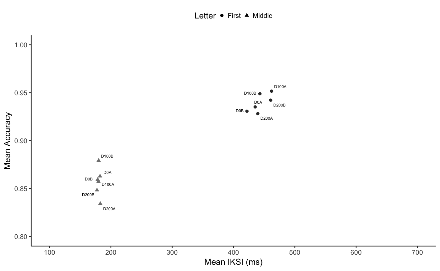
## -0.02695755

speed accuracy tradeoff

library(ggrepel)
E3_iksi_both <- rbind(E3_FL_iksi_table,
                       E3_ML_iksi_table)

E3_iksi_both <- cbind(E3_iksi_both, 
                       Letter_Position = rep(c("First","Middle"), each=6))

E3_acc_both <- rbind(E3acc_FL_table,
                       E3acc_ML_table)

E3_acc_both <- cbind(E3_acc_both, 
                       Letter_Position = rep(c("First","Middle"), each=6))

E3_SA <- cbind(E3_iksi_both, accuracy = E3_acc_both$mAcc)

E3_SA_graph <- ggplot(E3_SA, aes(x=mIKSI,  y=accuracy,
                   shape=Letter_Position,
                   color=Letter_Position,
                   label=delay))+
  geom_point()+
  geom_text_repel(size=1.7, color="black")+
  coord_cartesian(xlim=c(100,700), ylim=c(.8,1))+
  scale_x_continuous(breaks=seq(100,700,100))+
  scale_color_grey(start = 0.2, end = 0.5, na.value = "red",
  aesthetics = "color", guide =FALSE)+
  theme_classic(base_size=10)+
  ylab("Mean Accuracy")+
  xlab("Mean IKSI (ms)")+
  #facet_wrap(~Letter_Position, nrow=2,
  #           strip.position="right")+
  theme(legend.position ="top",
        legend.direction = "horizontal")+
  guides(shape = guide_legend(label.hjust = 0,
                              keywidth=0.1))+
  labs(shape="Letter")
  

E3_SA_graph

Save all

save.image(file="E3_workspace.RData")