Show the code
library(tidyverse)
library(openai)
library(patchwork)
library(xtable)Matthew J. C. Crump 
Simulation 1 showed that several aspects of trial-to-trial performance in a Stroop task can be simulated by gpt-3.5-turbo. However, some aspects of performance were too good to be human. First, the model produced perfect responses on all trials. Second, the simulated reaction time values were too round, and usually ended in zero or five. Simulation 2 determines whether changes to the prompt instructions can deliver different patterns of results. The prompt will include instructions to perform with accuracy rates between 85% and 95%. The prompt will also include instructions to generate reaction time results that end in any number.
library(tidyverse)
library(openai)
library(patchwork)
library(xtable)Notes: 25 simulated subjects. 24 Stroop trials each. 50% congruent/incongruent items made up from combinations of red, green, blue, and yellow.
The new prompt is shown in the code.
Timing it this time. Started at 3:10. Took about 14 minutes.
Used default params for gpt-3.5-turbo from the openai library.
# use the colors red, green, blue, and yellow

# four possible congruent items
congruent_items <- c("The word red printed in the color red",
                     "The word blue printed in the color blue",
                     "The word yellow printed in the color yellow",
                     "The word green printed in the color green")

# four possible incongruent items
incongruent_items <- c("The word red printed in the color blue",
                       "The word red printed in the color green",
                       "The word red printed in the color yellow",
                       "The word blue printed in the color red",
                       "The word blue printed in the color green",
                       "The word blue printed in the color yellow",
                       "The word yellow printed in the color red",
                       "The word yellow printed in the color blue",
                       "The word yellow printed in the color green",
                       "The word green printed in the color red",
                       "The word green printed in the color blue",
                       "The word green printed in the color yellow")

# generate 50% congruent and 50% incongruent trials
# 12 each (congruent and incongruent)
trials <- sample(c(rep(congruent_items,3),incongruent_items))


#set up variables to store data
all_sim_data <- tibble()
gpt_response_list <- list()

# request multiple subjects
# submit a query to open ai using the following prompt
# note: responses in JSON format are requested

for(i in 1:25){
  print(i)

  gpt_response <- create_chat_completion(
   model = "gpt-3.5-turbo",
   messages = list(
       list(
           "role" = "system",
           "content" = "You are a simulated participant in a human cognition experiment. Complete the task as instructed and record your simulated responses in a JSON file"),
       list("role" = "assistant",
            "content" = "OK, I am ready."),
       list("role" = "user",
           "content" = paste("Consider the following trials of a Stroop task where you are supposed to identify the ink-color of the word as quickly and accurately as possible.","-----", paste(1:24, trials, collapse="\n") , "-----",'This is a simulated Stroop task. You will be shown a Stroop item in the form of a sentence. The sentence will describe a word presented in a particular ink-color. Your task is to identify the ink-color of the word as quickly and accurately as a human participant would. Your simulated accuracy should be between 80 and 95 percent accurate. Your simulated reaction times should look like real human data and end in different numbers. Put the simulated identification response and reaction time into a JSON array using this format: [{"trial": "trial number, integer", "word": "the name of the word, string","color": "the color of the word, string","response": "the simulated identification response, string","reaction_time": "the simulated reaction time, milliseconds an integer"}].', sep="\n")

       )
   )
)

  # save the output from openai
  gpt_response_list[[i]] <- gpt_response

  # validate the JSON
  test_JSON <- jsonlite::validate(gpt_response$choices$message.content)

  # validation checks pass, write the simulated data to all_sim_data
  if(test_JSON == TRUE){
    sim_data <- jsonlite::fromJSON(gpt_response$choices$message.content)

    if(sum(names(sim_data) == c("trial","word","color","response","reaction_time")) == 5) {
      sim_data <- sim_data %>%
        mutate(sim_subject = i)

      all_sim_data <- rbind(all_sim_data,sim_data)
    }

  }
}

# model responses are in JSON format
save.image("data/simulation_2.RData")load(file = "data/simulation_2.RData")The LLM occasionally returns invalid JSON. The simulation ran 25 times, but still need to compute the total number of valid simulated subjects.
total_subjects <- length(unique(all_sim_data$sim_subject))There were 25 out of 25 valid simulated subjects.
# get mean RTs in each condition for each subject
rt_data_subject_congruency <- all_sim_data %>%
  mutate(congruency = case_when(word == color ~ "congruent",
                                word != color ~ "incongruent")) %>%
  mutate(accuracy = case_when(response == color ~ TRUE,
                              response != color ~ FALSE)) %>%
  filter(accuracy == TRUE) %>%
  group_by(congruency,sim_subject) %>%
  summarize(mean_rt = mean(reaction_time), .groups = "drop")

# Compute difference scores for each subject
rt_data_subject_stroop <- rt_data_subject_congruency %>%
  pivot_wider(names_from = congruency,
              values_from = mean_rt) %>%
  mutate(Stroop_effect = incongruent-congruent)

# make plots

F1A <- ggplot(rt_data_subject_congruency, aes(x = congruency,
                                       y = mean_rt))+
  geom_violin()+
  stat_summary(fun = "mean",
               geom = "crossbar",
               color = "red")+
  geom_point()+
  theme_classic(base_size=15)+
  ylab("Mean Simulated Reaction Time") +
  ggtitle("A")

F1B <- ggplot(rt_data_subject_stroop, aes(x = ' ',
                                   y = Stroop_effect))+
  geom_violin()+
  stat_summary(fun = "mean",
               geom = "crossbar",
               color = "red")+
  geom_point()+
  theme_classic(base_size=15)+
  ylab("Simulated Stroop Effects")+
  xlab("Incongruent - Congruent")+
  ggtitle("B")

F1A + F1B
Figure 1A shows simulated mean reaction times for congruent and incongruent trials. Individual dots show means at the level of simulated subjects. Figure 1B shows the overall mean Stroop effect and individual mean Stroop effects for each simulated subject. The results are similar to Simulation 1.
The new prompt included the instructions: “Your simulated accuracy should be between 80 and 95 percent accurate. Your simulated reaction times should look like real human data and end in different numbers.” A major question for simulation 2 was to determine if this prompt would cause the model to generate less round numbers.
The histogram looks more like an ex-Gaussian than simulation 1.
ggplot(all_sim_data, aes(x=reaction_time))+
  geom_histogram(binwidth=50, color="white")+
  theme_classic()+
  xlab("Simulated Reaction Times")
Setting the bin-width smaller shows that the model used many more numbers in between round intervals.
ggplot(all_sim_data, aes(x=reaction_time))+
  geom_histogram(binwidth=10, color="white")+
  scale_x_continuous(breaks=seq(250,1000,50))+
  theme_classic(base_size = 10)+
  xlab("Simulated Reaction Times")
The following histogram is a count of the ending digits for each of the simulated reaction times generated by gpt-3.5-turbo. The new prompt was effective in causing the model to produce numbers with all possible endings.
all_sim_data <- all_sim_data %>%
  mutate(ending_digit = stringr::str_extract(all_sim_data$reaction_time, "\\d$")) %>%
  mutate(ending_digit = as.numeric(ending_digit))

ggplot(all_sim_data, aes(x=ending_digit))+
  geom_histogram(binwidth=1, color="white")+
  scale_x_continuous(breaks=seq(0,9,1))+
  theme_classic(base_size = 10)+
  xlab("Simulated RT Ones Digit")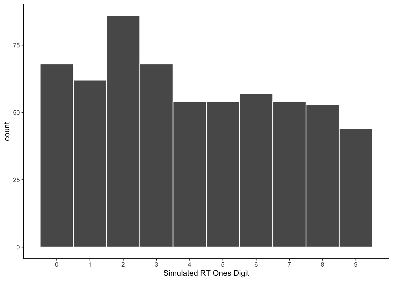
Another major question was whether the new prompt would cause less than perfect accuracy on all trials. The model remained 100% accurate on congruent trials, but produced a variety of accuracy rates for incongruent trials.
# report accuracy data
accuracy_data_subject <- all_sim_data %>%
  mutate(congruency = case_when(word == color ~ "congruent",
                                word != color ~ "incongruent")) %>%
  mutate(accuracy = case_when(response == color ~ TRUE,
                              response != color ~ FALSE)) %>%
  group_by(congruency,sim_subject) %>%
  summarize(proportion_correct = sum(accuracy)/12, .groups = "drop")

ggplot(accuracy_data_subject, aes(x = congruency,
                                  y = proportion_correct))+
  geom_violin()+
  stat_summary(fun = "mean",
               geom = "crossbar",
               color = "red")+
  geom_point()+
  theme_classic(base_size=15)+
  ylab("Simulated Proportion Correct")+
  xlab("Congruency")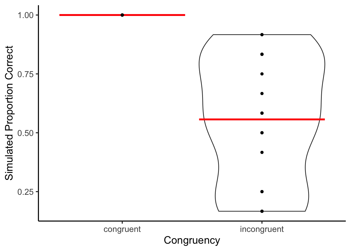
The accuracy rates for incongruent items have a clear stepped, almost equal interval like pattern. The prompt succeeded in producing imperfect accuracy rates, but the model did not comply with the instruction to produce accuracy rates between 80-95 percent correct.
The purpose of Simulation 2 was to determine if simple changes to the instructions would influence the simulated results. The goal was to produce reaction times that appeared more random and ex-Gaussian, as well as more inaccurate responses. In Simulation 2, the reaction times were indeed more random and ex-Gaussian compared to Simulation 1. While the accuracy rates for congruent items remained perfect, there was a wide range of accuracy rates for incongruent items.