Show the code
library(tidyverse)
library(openai)
library(patchwork)
library(xtable)Matthew J. C. Crump 
Started. Finished
The previous simulations focused on the Stroop task. This simulation uses a version of the Eriksen Flanker task.
library(tidyverse)
library(openai)
library(patchwork)
library(xtable)Notes: 15 simulated subjects. 20 Flanker trials each. 50/50 congruent and incongruent trials.
The prompt is given only basic information to complete the task.
Used gpt-3.5-turbo-16k, with max tokens 10000.
Problems: Still getting the occasional invalid JSON back, mostly due to the chatbot prefacing its response with a message before the JSON. This thread may be helpful https://community.openai.com/t/getting-response-data-as-a-fixed-consistent-json-response/28471/31?page=2.
# Use letters H and F

compatible_items <- data.frame(stimulus = c("HHHHH",
                                           "FFFFF"),
                               response = "?",
                               reaction_time = "?")

incompatible_items <- data.frame(stimulus = c("FFHFF",
                                           "HHFHH"),
                                 response = "?",
                                 reaction_time = "?")


#set up variables to store data
all_sim_data <- tibble()
gpt_response_list <- list()

# request multiple subjects
# submit a query to open ai using the following prompt
# note: responses in JSON format are requested

for(i in 1:15){
  print(i)

  # construct trials data frame
  compatible_trials <- compatible_items[rep(1:nrow(compatible_items),5),]
  incompatible_trials <- incompatible_items[rep(1:nrow(incompatible_items),5),]

  trials <- rbind(compatible_trials,
                  incompatible_trials
                  ) %>%
    mutate(instruction = "Identify center letter")

  trials <- trials[sample(1:nrow(trials)),]
  trials <- trials %>%
    mutate(trial = 1:nrow(trials)) %>%
    relocate(instruction) %>%
    relocate(trial)

   # run the api call to openai

 gpt_response <- create_chat_completion(
   model = "gpt-3.5-turbo-16k",
   max_tokens = 10000,
   messages = list(
       list(
           "role" = "system",
           "content" = "You are a simulated participant in a human cognition experiment. Complete the task as instructed and record your simulated responses in a JSON file. Do not include any explanations, only provide a RFC8259 compliant JSON response."),
       list("role" = "assistant",
            "content" = "OK, I am ready."),
       list("role" = "user",
           "content" = paste('You are a simulated participant in a human cognition experiment. Complete the task as instructed and record your simulated responses in JSON. Your task is to simulate human performance in a letter identification task. You will be given the task in the form a JSON object. The JSON object contains the task instruction and the stimulus on each trial. Your task is to follow the instruction and respond to the stimulus as quickly and accurately as a human participant would. When you simulate data make sure it conforms to how humans would perform this task. The JSON object contains the symbol ? in locations where you will generate simulated responses. You will generate a simulated identification response, and a simulated reaction time for each trial. Put the simulated identification response and reaction time into a JSON array using this format: [{"trial": "trial number, integer", "instruction" = "the task instruction, string", "stimulus": "the stimulus, string","response": "the simulated identification response, string","reaction_time": "the simulated reaction time, milliseconds an integer"}].', "\n\n", jsonlite::toJSON(trials), collapse = "\n")

       )
   )
)

  # save the output from openai
  gpt_response_list[[i]] <- gpt_response
  print(gpt_response$usage$total_tokens)

  # validate the JSON
  test_JSON <- jsonlite::validate(gpt_response$choices$message.content)
  print(test_JSON)

  # validation checks pass, write the simulated data to all_sim_data
  if(test_JSON == TRUE){
    sim_data <- jsonlite::fromJSON(gpt_response$choices$message.content)

    if(sum(names(sim_data) == c("trial","instruction","stimulus","response","reaction_time")) == 5) {

      sim_data <- sim_data %>%
        mutate(sim_subject = i)

      all_sim_data <- rbind(all_sim_data,sim_data)
    }

  }
}

# model responses are in JSON format
save.image("data/simulation_9.RData")load(file = "data/simulation_9.RData")The LLM occasionally returns invalid JSON. The simulation ran 15 times.
total_subjects <- length(unique(all_sim_data$sim_subject))There were 14 out of 15 valid simulated subjects.
all_sim_data <- all_sim_data %>%
  mutate(reaction_time = as.numeric(reaction_time))

# get mean RTs in each condition for each subject
rt_data_subject_congruency <- all_sim_data %>%
  mutate(congruency = case_when(stimulus %in% c("HHHHH","FFFFF") ~ "congruent",
                                stimulus %in% c("HHFHH","FFHFF") ~ "incongruent")
         )%>%
  rowwise() %>%
  mutate(center_letter = stringr::str_split(stimulus,"")[[1]][3]) %>%
  as.data.frame() %>%
  mutate(accuracy = case_when(center_letter == response ~ TRUE,
                              center_letter != response ~ FALSE
                              )
         ) %>%
  filter(accuracy == TRUE) %>%
  group_by(congruency,sim_subject) %>%
  summarize(mean_rt = mean(reaction_time), .groups = "drop")


# Compute difference scores for each subject
rt_data_subject_flanker <- rt_data_subject_congruency %>%
  pivot_wider(names_from = congruency,
              values_from = mean_rt) %>%
  mutate(Flanker_effect = incongruent-congruent)

# make plots

F1A <- ggplot(rt_data_subject_congruency, aes(x = congruency,
                                       y = mean_rt))+
  geom_violin()+
  stat_summary(fun = "mean",
               geom = "crossbar",
               color = "red")+
  geom_point()+
  theme_classic(base_size=15)+
  ylab("Mean Simulated Reaction Time") +
  ggtitle("A")

F1B <- ggplot(rt_data_subject_flanker, aes(x = ' ',
                                   y = Flanker_effect))+
  geom_violin()+
  stat_summary(fun = "mean",
               geom = "crossbar",
               color = "red")+
  geom_point()+
  theme_classic(base_size=15)+
  ylab("Simulated Flanker Effects")+
  xlab("Incongruent - Congruent")+
  ggtitle("B")

F1A + F1B
The figure shows that mean reaction times were faster for congruent than incongruent flanker items. Also, 11 out of 14 simulated subjects showed a positive flanker effect.
Here is a histogram of the individual simulated reaction times.
ggplot(all_sim_data, aes(x=reaction_time))+
  geom_histogram(binwidth=50, color="white")+
  theme_classic()+
  xlab("Simulated Reaction Times")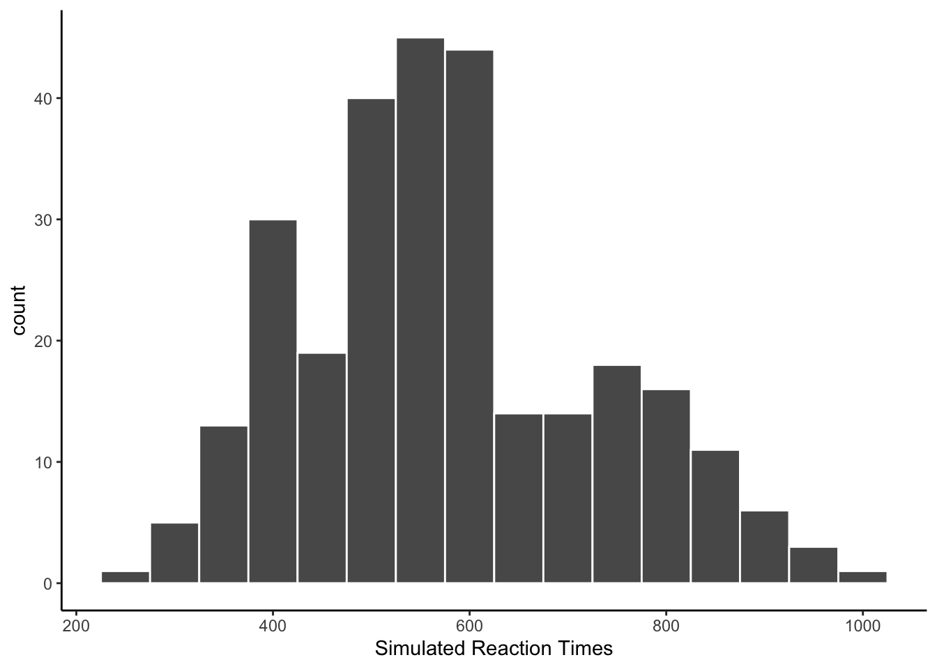
The prompt did not specify to produce values with different endings. As with previous simulations, the model prefers values ending in 0.
all_sim_data <- all_sim_data %>%
  mutate(ending_digit = stringr::str_extract(all_sim_data$reaction_time, "\\d$")) %>%
  mutate(ending_digit = as.numeric(ending_digit))

ggplot(all_sim_data, aes(x=ending_digit))+
  geom_histogram(binwidth=1, color="white")+
  scale_x_continuous(breaks=seq(0,9,1))+
  theme_classic(base_size = 10)+
  xlab("Simulated RT Ones Digit")
The model performs perfectly on congruent trials, and sometimes imperfectly on incongruent trials.
# report accuracy data
accuracy_data_subject <- all_sim_data %>%
  mutate(congruency = case_when(stimulus %in% c("HHHHH","FFFFF") ~ "congruent",
                                stimulus %in% c("HHFHH","FFHFF") ~ "incongruent")
         )%>%
  rowwise() %>%
  mutate(center_letter = stringr::str_split(stimulus,"")[[1]][3]) %>%
  as.data.frame() %>%
  mutate(accuracy = case_when(center_letter == response ~ TRUE,
                              center_letter != response ~ FALSE
                              )
         ) %>%
  group_by(congruency,sim_subject) %>%
  summarize(proportion_correct = mean(accuracy), .groups = "drop")

ggplot(accuracy_data_subject, aes(x = congruency,
                                  y = proportion_correct))+
  geom_violin()+
  stat_summary(fun = "mean",
               geom = "crossbar",
               color = "red")+
  geom_point()+
  theme_classic(base_size=15)+
  ylab("Simulated Proportion Correct")+
  xlab("Congruency")
This simulation produced results that reflected patterns in Flanker data, especially at the level of group and subject means. Individual reaction times are again too round (ending in zero). Accuracy rates are too perfect for congruent items.
It remains frustrating that the GPT model is stochastic, and that these results are not reproducible. I could run several batches with larger N to determine whether this result is somewhat stable, but this wouldn’t guarantee the same results could be produced at a later date because the underlying model may change at any time.